okama.Portfolio.plot_forecast

Portfolio.plot_forecast(distr='norm', years=5, percentiles=[10, 50, 90], today_value=None, n=1000, figsize=None)

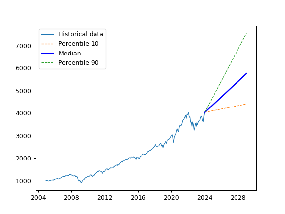
Plot forecasted ranges of wealth indexes (lines) for a given set of percentiles. Historical wealth index is shown in the same chart.

Parameters:

distr{‘hist’, ‘norm’, ‘lognorm’}, default ‘norm’

Distribution type for the rate of return of portfolio. ‘norm’ - for normal distribution. ‘lognorm’ - for lognormal distribution. ‘hist’ - percentiles are taken from the historical data.

yearsint, default 1

Investment period length to calculate wealth index. It should not exceed 1/2 of the portfolio history period length ‘period_length’.

percentileslist of int, default [10, 50, 90]

List of percentiles to be calculated.

today_valueint, optional

Initial value of the wealth index. If today_value is None the last value of the historical wealth indexes is taken. It can be useful to plot the forecast of wealth index togeather with the hitorical data.

nint, default 1000

Number of random time series to generate with Monte Carlo simulation (for ‘norm’ or ‘lognorm’ only). Larger argument values can be used to increase the precision of the calculation. But this will lead to slower performance. Is not required for historical distribution (dist=’hist’).

Returns:

Axes‘matplotlib.axes._subplots.AxesSubplot’

Examples

>>> import matplotlib.pyplot as plt
>>> pf = ok.Portfolio(['SPY.US', 'AGG.US', 'GLD.US'], weights=[.60, .35, .05], rebalancing_period='year')
>>> pf.plot_forecast()
>>> plt.show()