You can run the code examples in Google Colab.
To install the package:
[ ]:
!pip install okama
import okama and matplotlib packages …
[1]:
import warnings

import matplotlib.pyplot as plt

plt.rcParams["figure.figsize"] = [12.0, 6.0]
warnings.simplefilter(action='ignore', category=FutureWarning)

import okama as ok
Portfolio and AssetList can be helpful to learn about investment portfolio properties and to compare various portfolios with each other. With AssetList we can even compare portfolio with stocks, indexes and other types of financial assets (portfolio is just a special case of a financial asset).
In this tutorial we will learn how to:
Create investment portfolio and see its basic properties
Rebalancing strategy and asset allocation
Risk metrics of the portfolio
Accumulated return, CAGR and dividend yield
Compare several portfolios
Forecast portfolios performance
Create an investment portfolio
Portfolios are quite similar to AssetList, but we should specify weights and rebalancing strategy.
All the arguments have default values and can be skipped.
[2]:
basic_portfolio = ok.Portfolio()
basic_portfolio
[2]:
symbol                 portfolio_6059.PF
assets                          [SPY.US]
weights                            [1.0]
rebalancing_period                 month
currency                             USD
inflation                       USD.INFL
first_date                       1993-02
last_date                        2024-01
period_length         31 years, 0 months
dtype: object
inflation=TrueRebalancing is the process by which an investor restores their portfolio to its target allocation by selling and buying assets. After rebalancing all the assets have original weights.
rebalancing_period attribute can be: ‘month’, ‘year’, ‘half-year’, ‘quarter’ or ‘none’ (for not rebalanced portfolios).
[3]:
rf3 = ok.Portfolio(
    ["BND.US", "VTI.US", "VXUS.US"],
    weights=[0.40, 0.40, 0.20],
    rebalancing_period="year",
)
rf3
[3]:
symbol                        portfolio_8142.PF
assets                [BND.US, VTI.US, VXUS.US]
weights                         [0.4, 0.4, 0.2]
rebalancing_period                         year
currency                                    USD
inflation                              USD.INFL
first_date                              2011-02
last_date                               2024-01
period_length                13 years, 0 months
dtype: object
.assets_first_dates and .assets_last_dates[4]:
rf3.assets_first_dates
[4]:
{'USD': Timestamp('1913-02-01 00:00:00'),
 'VTI.US': Timestamp('2001-06-01 00:00:00'),
 'BND.US': Timestamp('2007-05-01 00:00:00'),
 'VXUS.US': Timestamp('2011-02-01 00:00:00'),
 'USD.INFL': Timestamp('1913-02-01 00:00:00')}
[5]:
rf3.newest_asset
[5]:
'VXUS.US'
Here VXUS.US is a stock with the shortest history which is limiting the whole portfolio data.
[6]:
rf3.assets_last_dates
[6]:
{'BND.US': Timestamp('2024-02-01 00:00:00'),
 'VTI.US': Timestamp('2024-02-01 00:00:00'),
 'VXUS.US': Timestamp('2024-02-01 00:00:00'),
 'USD': Timestamp('2099-12-01 00:00:00'),
 'USD.INFL': Timestamp('2024-01-01 00:00:00')}
On the other hand, the inflation is limiting the data from the left side. If you need last month’s data to be included inflation=False should be used in Portfolio instantiating.
symbol= in portfolio instantiating or set it afterwards:[7]:
rf3.symbol = "RF3_portfolio.PF" # 'PF' namespace is reserved for portfolios.
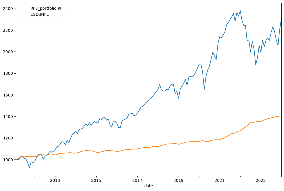
Wealth index (Cumulative Wealth Index) is a time series that presents the value of portfolio over historical time period. The initial investment is 1000 points in a base currency.
[8]:
rf3.wealth_index.plot();
Rebalancing strategy and asset allocaction
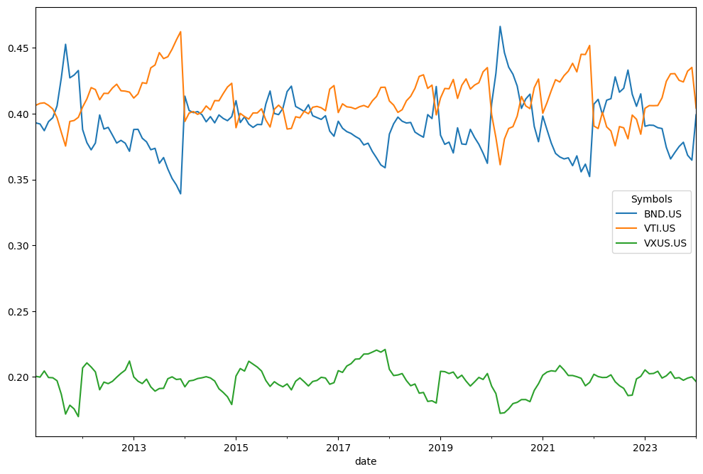
Table with original asset allocation can be seen with .table:
[9]:
rf3.table
[9]:
| asset name | ticker | weights | |
|---|---|---|---|
| 0 | Vanguard Total Bond Market Index Fund ETF Shares | BND.US | 0.4 |
| 1 | Vanguard Total Stock Market Index Fund ETF Shares | VTI.US | 0.4 |
| 2 | Vanguard Total International Stock Index Fund ... | VXUS.US | 0.2 |
.weights_ts:[10]:
rf3.weights_ts.plot();
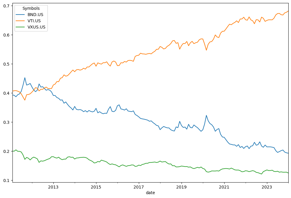
let’s create the same Rick Ferry portfolio, but without rebalancing (asset allocation will change and never return to the original weights).
[11]:
rf3_no_rebalancing = ok.Portfolio(
    ["BND.US", "VTI.US", "VXUS.US"],
    weights=[0.40, 0.40, 0.20],
    rebalancing_period="none",
)
Now it’s easy to see how the weights get out of control over time… and we end up with portfolio overweight in stocks.
[12]:
rf3_no_rebalancing.weights_ts.plot();
Risk metrics of the portfolio
Portfolio has several methods to see risk metrics. By default with ‘risk’ we understand return time series standard deviation:
risk_monthly (standard deviation for monthly rate of return time series)
risk_annual (annualized standart deviation)
semideviation_monthly (downside risk for monthly rate of return time series)
semideviation_annual (annualized semideviation)
get_var_historic (historic Value at Risk for the portfolio)
get_cvar_historic (historic Conditional Value at Risk for the portfolio)
drawdowns (percent decline from a previous peak)
recovery_period (the longest recovery period after drawdown for the portfolio assets value)
[13]:
rf3.risk_annual # aanualized value for standard deviation of return
[13]:
date
2011-03    0.001190
2011-04    0.061240
2011-05    0.055790
2011-06    0.053769
2011-07    0.048875
             ...
2023-09    0.098806
2023-10    0.098652
2023-11    0.100879
2023-12    0.101558
2024-01    0.101203
Freq: M, Name: RF3_portfolio.PF, Length: 155, dtype: float64
[14]:
rf3.semideviation_annual # annualized value for downside risk
[14]:
0.07626419142775892
[15]:
rf3.get_cvar_historic(time_frame=12, level=1) # one year CVAR with confidence level 1%
[15]:
0.17793338953579407
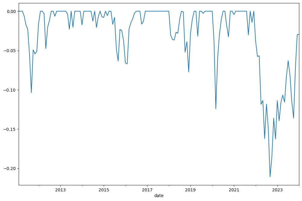
Drawdowns (the percent decline from a previous peak) are easy to plot …
[16]:
rf3.drawdowns.plot();
[17]:
rf3.drawdowns.nsmallest(5) # 5 Biggest drawdowns
[17]:
date
2022-09   -0.210563
2022-10   -0.185137
2022-12   -0.162683
2022-06   -0.162101
2022-08   -0.148924
Freq: M, Name: RF3_portfolio.PF, dtype: float64
reovery_period highly related with Drawdowns. It shows the longest recovery periods for the portfolio value after drawdowns.
[19]:
rf3.recovery_period.nlargest() / 12 # we want it in years
[19]:
date
2016-07    1.083333
2012-02    0.750000
2018-08    0.500000
2019-03    0.500000
2020-07    0.416667
Freq: M, Name: RF3_portfolio.PF, dtype: float64
Accumulated return, CAGR and dividend yield
Portfolio has several metrics to measure the profits and return:
wealth_index (the value of portfolio over historical time period)
wealth_index_with_assets (wealth index with assets values)
mean_return_monthly (arithmetic mean for the portfolio rate of return)
mean_return_annual (annualized value for monthly mean)
annual_return_ts (Annual rate of return time series)
get_cagr (Compound Annual Growth Rate for a given trailing period)
get_rolling_cagr (rolling CAGR with)
get_cumulative_return (cumulative return over a given trailing period)
get_rolling_cumulative_return (rolling cumulative return)
dividend_yield (portfolio LTM dividend yield monthly time series)
wealth_index_with_assets method.[20]:
rf3.wealth_index_with_assets.plot();
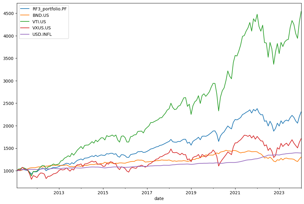
Mean reaturn (arithmetic mean) for the portfolio is an annualized version of monthly mean:
[21]:
rf3.mean_return_annual
[21]:
0.07289051506527566
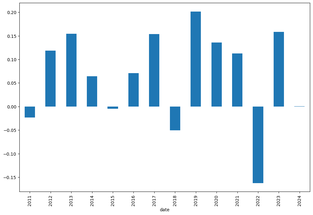
It’s always good to see how portfolio perform on annual basis. Annual rate of return time series show portfolio return for each calendar year:
[22]:
rf3.annual_return_ts
[22]:
date
2011   -0.023654
2012    0.118483
2013    0.154623
2014    0.063946
2015   -0.004685
2016    0.070988
2017    0.154072
2018   -0.050306
2019    0.201576
2020    0.135694
2021    0.112768
2022   -0.162683
2023    0.158682
2024    0.000420
Freq: Y-DEC, Name: RF3_portfolio.PF, dtype: float64
… or in form of bar chart:
[23]:
rf3.annual_return_ts.plot(kind="bar");
One of the most important return metrics is CAGR (Compound Annual Growth Rate). It can be seen for trailing periods (parameter period is in years):
[24]:
rf3.get_cagr(period=5) # portfolio is initiated with inflation=True. Hence, we see CAGR with mean inflation.
[24]:
RF3_portfolio.PF    0.069369
USD.INFL            0.041477
dtype: float64
[25]:
rf3.get_cagr(period=5, real=True) # when real=True CAGR is adjusted for inflation (real CAGR)
[25]:
RF3_portfolio.PF    0.02678
dtype: float64
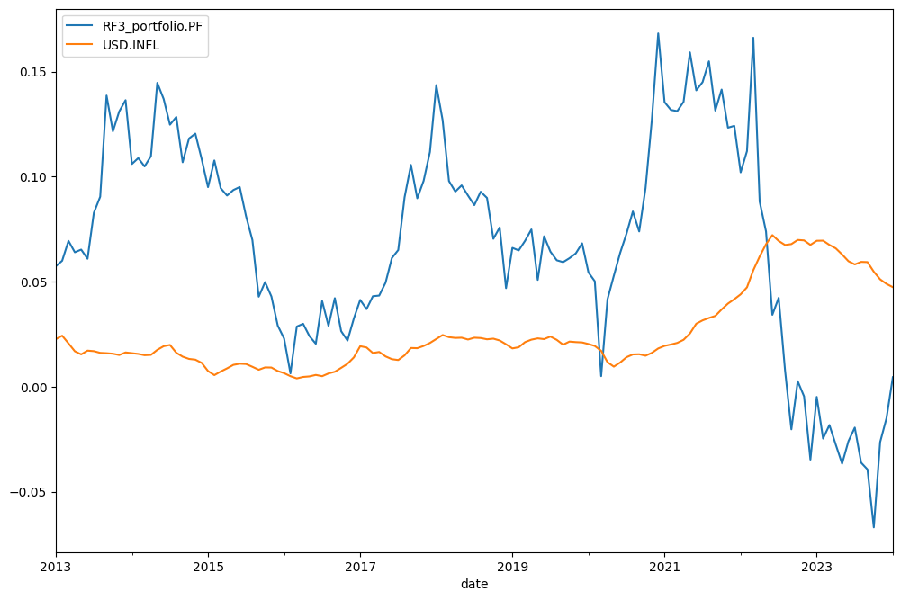
Rolling CAGR for the portfolio is available with get_rolling_cagr:
[26]:
rf3.get_rolling_cagr(
    window=12 * 2
).plot();  # window size is in moths. We have rolling 2 year CAGR here and rolling 2 year mean inflation ...
Cumulative return over a given trailing period can be calculated with get_cumulative_return. Period argument can be in years or YTD (Year To Date).
[27]:
rf3.get_cumulative_return(
    period="YTD"
)  # Return since the beginning of the current calendar year and the inflation for the same period
[27]:
RF3_portfolio.PF    0.00042
USD.INFL            0.00540
dtype: float64
[28]:
rf3.get_cumulative_return(period=5) # Cumulative return for the 5 years period
[28]:
RF3_portfolio.PF    0.398419
USD.INFL            0.225319
dtype: float64
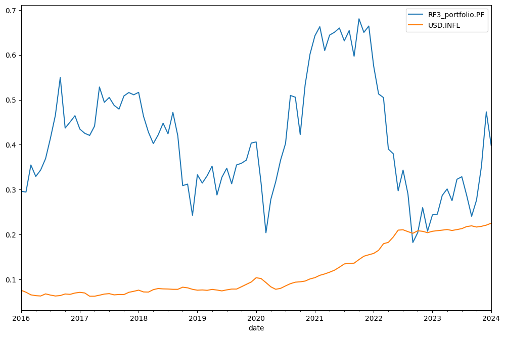
Cumulative rolling return can be helpfull in the same situation as rolling CAGR:
[29]:
rf3.get_rolling_cumulative_return(window=12 * 5).plot(); # window size is in months (5 year cumulative return here)
Last twelve months (LTM) dividend yield is available with dividend_yield property.
[30]:
rf3.dividend_yield.plot();
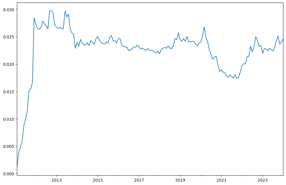
Portfolio has monthly dividends time series:
[31]:
rf3.dividends
[31]:
2011-02     1.101142
2011-03     2.716983
2011-04     1.090118
2011-05     1.104542
2011-06     2.827576
             ...
2023-09     8.201548
2023-10     2.238355
2023-11     2.151184
2023-12    15.014867
2024-01     0.000000
Freq: M, Name: RF3_portfolio.PF, Length: 156, dtype: float64
Calendar year dividends sum time series for the portfolio:
[32]:
rf3.dividends.resample("Y").sum().plot(kind="bar");
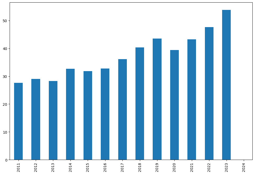
Sharpe Ratio was developed by Nobel laureate William F. Sharpe and is used to understand the return of an investment compared to its risk.
\[S_p = \frac{R_p - R_f}{\sigma_p}\]\(R_p\) - expected return of portfolio
[33]:
rf3.get_sharpe_ratio(rf_return=0.02) # risk-free rate is 2% here
[33]:
0.5226169918055219
Finally the easiest way to see the portfolio basic properties is with describe:
[34]:
rf3.describe()
[34]:
| property | period | RF3_portfolio.PF | inflation | |
|---|---|---|---|---|
| 0 | compound return | YTD | 0.00042 | 0.005400 |
| 1 | CAGR | 1 years | 0.095291 | 0.030894 |
| 2 | CAGR | 5 years | 0.069369 | 0.041477 |
| 3 | CAGR | 10 years | 0.064267 | 0.028047 |
| 4 | CAGR | 13 years, 0 months | 0.066522 | 0.026266 |
| 5 | Annualized mean return | 13 years, 0 months | 0.072891 | NaN |
| 6 | Dividend yield | LTM | 0.024576 | NaN |
| 7 | Risk | 13 years, 0 months | 0.101203 | NaN |
| 8 | CVAR | 13 years, 0 months | 0.177933 | NaN |
| 9 | Max drawdown | 13 years, 0 months | -0.210563 | NaN |
| 10 | Max drawdown date | 13 years, 0 months | 2022-09 | NaN |
Compare several portfolios
Portfolio is a kind of financial asset and can be included in AssetList to compare with other portfolios (assets or benchmarks).
Lets create Rick Ferri 4 assets portfolio and compare the behaviour with 3 assets portfolio.
[35]:
assets = ["BND.US", "VTI.US", "VXUS.US", "VNQ.US"]  # Vanguard REIT ETF (VNQ) is added.
weights = [0.40, 0.30, 0.24, 0.06]
To compare properly with RF3 portfolio the same rebalancing period should be chosen:
[36]:
rf4 = ok.Portfolio(
    assets=assets, weights=weights, rebalancing_period="year", symbol="RF4_portfolio.PF"
)  # we also give a custom name to portfolio with 'symbol' propety
rf4
[36]:
symbol                                 RF4_portfolio.PF
assets                [BND.US, VTI.US, VXUS.US, VNQ.US]
weights                          [0.4, 0.3, 0.24, 0.06]
rebalancing_period                                 year
currency                                            USD
inflation                                      USD.INFL
first_date                                      2011-02
last_date                                       2024-01
period_length                        13 years, 0 months
dtype: object
Now we create an AssetList to compare RF3 with RF4 and add a benchamrk (SP 500 TR index).
[37]:
ls = ok.AssetList(["SP500TR.INDX", rf3, rf4])
ls
[37]:
assets           [SP500TR.INDX, RF3_portfolio.PF, RF4_portfolio...
currency                                                       USD
first_date                                                 2011-02
last_date                                                  2024-01
period_length                                   13 years, 0 months
inflation                                                 USD.INFL
dtype: object
Some behavior will be seen with wealth_indexes:
[38]:
ls.wealth_indexes.plot();
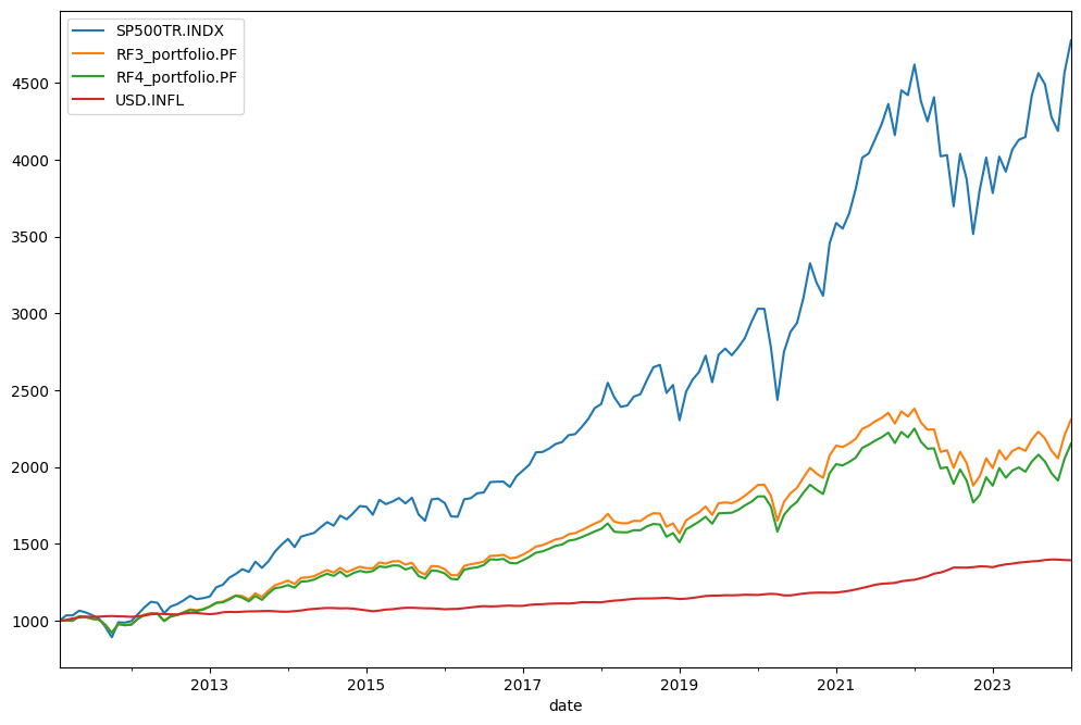
It worth plotting the portfolios and benchmark on the risk / return chart with plot_assets. X-axis is Risk (Standard Deviation) Y-axis is Return (Mean return or CAGR)
[39]:
ls.plot_assets(kind="cagr"); # we chouse CAGR (geomtric mean of return) as Y-axis by setting kind='cagr'
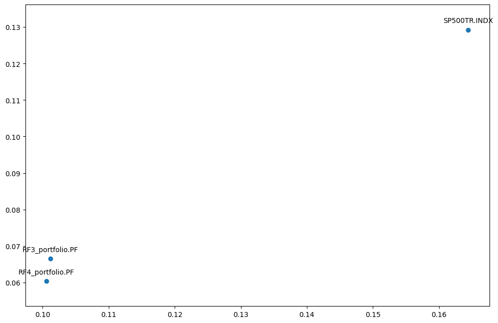
See04 efficient frontier single period.ipynband05 efficient frontier multi-period.ipynbto plot portfolios with the Efficient Frontier.
Given risk-free rate it’s easy to compare Sharpe Ratios of the portfolios and match it with the benchmark with get_sharpe_ratio:
[40]:
ls.get_sharpe_ratio(rf_return=0.02) # Risk-Free rate is 2% here
[40]:
Symbols
SP500TR.INDX        0.735977
RF3_portfolio.PF    0.506712
RF4_portfolio.PF    0.448621
dtype: float64
describe method.YTD (Year To date) compound return
CAGR for a given list of periods and full available period
Annualized mean rate of return (arithmetic mean)
LTM Dividend yield - last twelve months dividend yield
Risk metrics (full period):
risk (standard deviation)
CVAR (timeframe is 1 year)
max drawdowns (and dates of the drawdowns)
[42]:
ls.describe([1, 5, 8]) # portfolio CAGR is shown for YTD, 1, 5, 8 years and for the full histrical period.
[42]:
| property | period | SP500TR.INDX | RF3_portfolio.PF | RF4_portfolio.PF | inflation | |
|---|---|---|---|---|---|---|
| 0 | Compound return | YTD | 0.0168 | 0.00042 | -0.00442 | 0.0054 |
| 1 | CAGR | 1 years | 0.20806 | 0.095291 | 0.075325 | 0.030894 |
| 2 | CAGR | 5 years | 0.143037 | 0.069369 | 0.0609 | 0.041477 |
| 3 | CAGR | 8 years | 0.142018 | 0.074863 | 0.067389 | 0.033519 |
| 4 | CAGR | 13 years, 0 months | 0.129258 | 0.066522 | 0.060392 | 0.026266 |
| 5 | Annualized mean return | 13 years, 0 months | 0.141007 | 0.071281 | 0.06512 | NaN |
| 6 | Dividend yield | LTM | 0.0 | 0.023325 | 0.025546 | NaN |
| 7 | Risk | 13 years, 0 months | 0.164416 | 0.101203 | 0.100575 | NaN |
| 8 | CVAR | 13 years, 0 months | 0.167821 | 0.177933 | 0.181797 | NaN |
| 9 | Max drawdowns | 13 years, 0 months | -0.238631 | -0.210563 | -0.213989 | NaN |
| 10 | Max drawdowns dates | 13 years, 0 months | 2022-09 | 2022-09 | 2022-09 | NaN |
| 11 | Inception date | None | 1988-02 | 2011-02 | 2011-02 | 2011-02 |
| 12 | Last asset date | None | 2024-02 | 2024-01 | 2024-01 | 2024-01 |
| 13 | Common last data date | None | 2024-01 | 2024-01 | 2024-01 | 2024-01 |
Forecast portfolios performance
Forecasting methods are described in a dedicated notebook 07 forecasting.ipynb.
[ ]: