You can run the code examples in Google Colab.

To install the package:

[ ]:

!pip install okama

import okama and matplotlib packages …

[2]:

import matplotlib.pyplot as plt

plt.rcParams["figure.figsize"] = [12.0, 6.0]

import okama as ok

AssetList has a set of methods usefull to track perfomance of index funds and compare them with benchmarks: - tracking difference - tracking error - beta - rolling and cumulative correlations

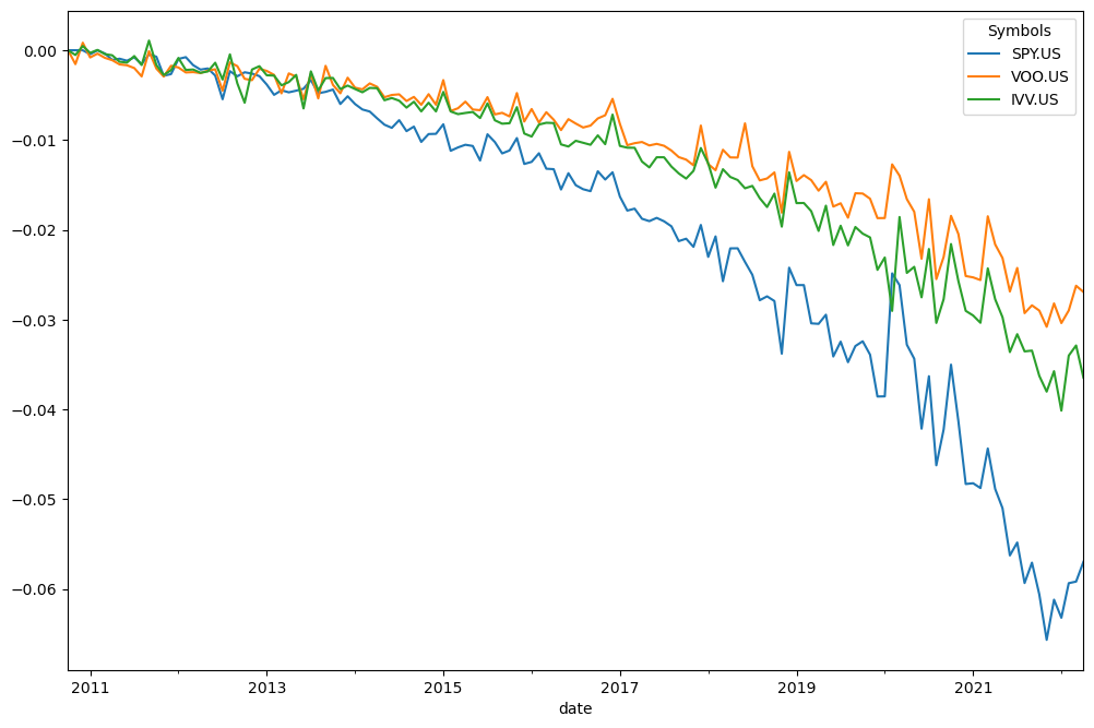
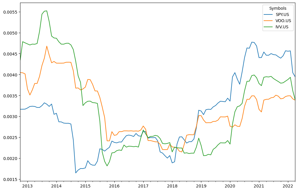
Tracking difference

Tracking diffrenece is calculated by measuring the difference between the accumulated return of an index and those of the ETFs replicating it.

Let’s compare main S&P500 ETFs.

[3]:

symbols = [
    "SP500TR.INDX",
    "SPY.US",
    "VOO.US",
    "IVV.US",
]  # the benchmark symbol should be in the first place
sp = ok.AssetList(symbols, last_date="2022-04")
sp

[3]:

assets           [SP500TR.INDX, SPY.US, VOO.US, IVV.US]
currency                                            USD
first_date                                      2010-10
last_date                                       2022-04
period_length                        11 years, 7 months
inflation                                      USD.INFL
dtype: object

[4]:

sp.names

[4]:

{'SP500TR.INDX': 'S&P 500 TR (Total Return)',
 'SPY.US': 'SPDR S&P 500 ETF Trust',
 'VOO.US': 'Vanguard S&P 500 ETF',
 'IVV.US': 'iShares Core S&P 500 ETF'}

We can check the general tracking difference as a difference in their accumulated return.

[5]:

sp.tracking_difference().plot();

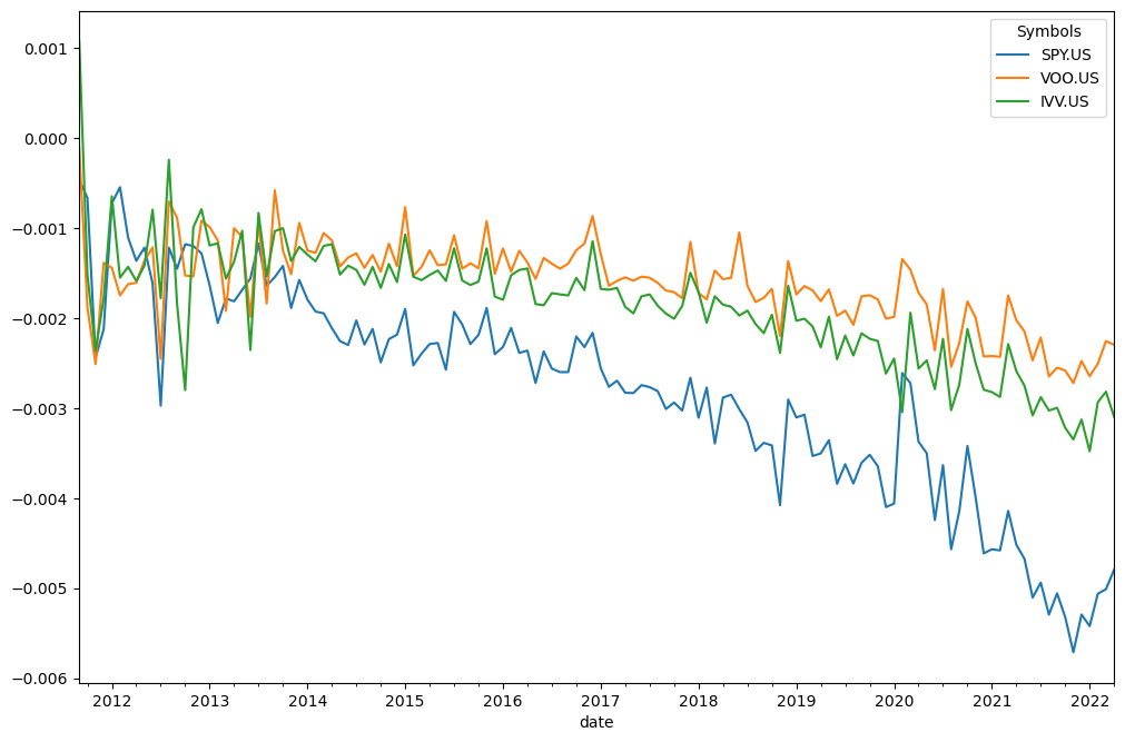
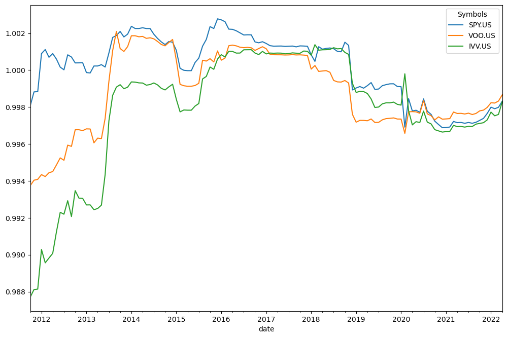
… or see annualized values.

[6]:

sp.tracking_difference_annualized().plot();

However above tracking difference includes 11 years of hisotrical data. Sometimes it’s useful to see the latest performance …

Use rolling tracking difference for that purpose:

[7]:

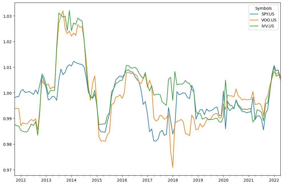
sp.tracking_difference_annualized(rolling_window=5 * 12).plot()  # rolling window is 5 years

[7]:

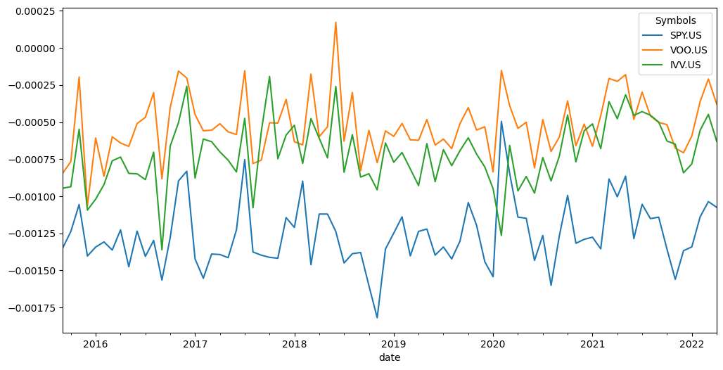
<AxesSubplot: xlabel='date'>

rolling_window parameter is also available in tracking_error(), index_beta() and index_correlation() functions.

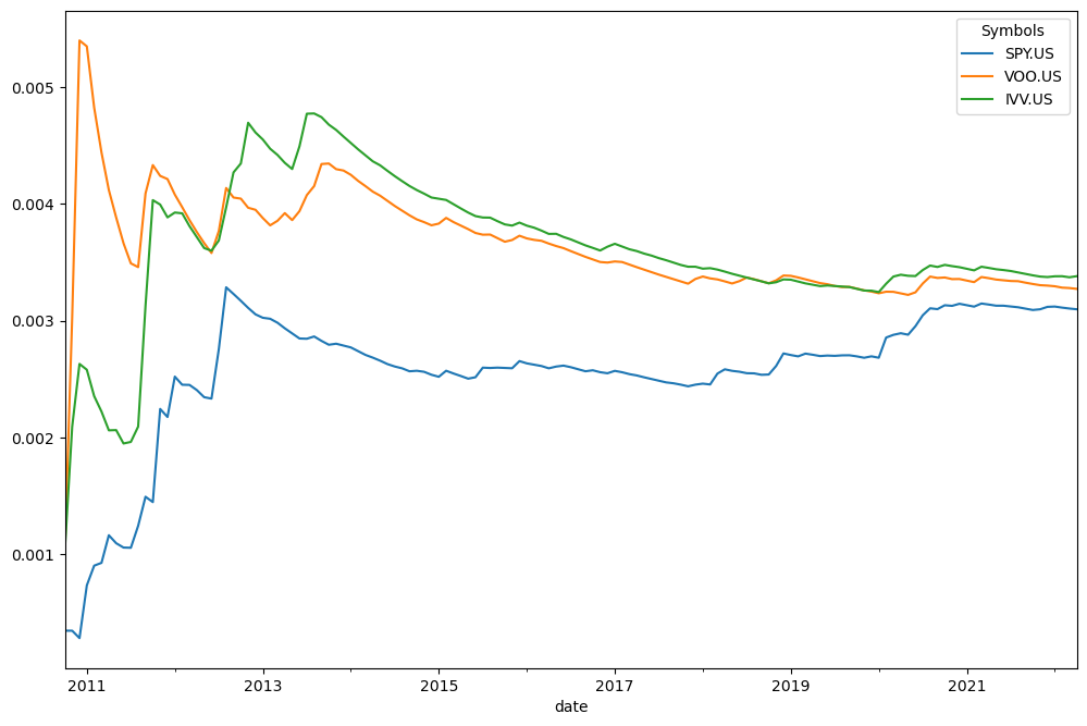
Tracking Error

Tracking Error is the standard deviation of the difference between the ETF and index returns.

[8]:

sp.tracking_error().plot();

… or rolling tracking error:

[9]:

sp.tracking_error(rolling_window=12 * 2).plot();

Beta

Another popular parameter for index funds is their beta.

The beta (β) of an asset (i.e. a stock) is a measurement of its volatility of returns relative to the entire market.

[10]:

sp.index_beta().plot();  # in this example as expected beta is close to 1. Each ETF represents broad market in form of S&P 500 index

… we see here that all 3 funds have similar beta.

Rolling beta is also available:

[12]:

sp.index_beta(rolling_window=12).plot();

Correlation with index

Sometimes it’s useful to check the correlation between different asset types.

In this example we verify the correlation:

US stocks (S&P 500 index)
US bonds (Vanguard mutual fund)
gold (spot prices)
US Real Estate (REIT ETF)

[13]:

assets = ["SP500TR.INDX", "VBMFX.US", "GC.COMM", "VNQ.US"]  # GC.COMM - gold spot prices
x = ok.AssetList(assets)
x

[13]:

assets           [SP500TR.INDX, VBMFX.US, GC.COMM, VNQ.US]
currency                                               USD
first_date                                         2004-10
last_date                                          2023-04
period_length                           18 years, 7 months
inflation                                         USD.INFL
dtype: object

[14]:

x.names

[14]:

{'SP500TR.INDX': 'S&P 500 TR (Total Return)',
 'VBMFX.US': 'VANGUARD TOTAL BOND MARKET INDEX FUND INVESTOR SHARES',
 'GC.COMM': 'Gold (COMEX)',
 'VNQ.US': 'Vanguard Real Estate Index Fund ETF Shares'}

It is possible to see as the correlation was changing during the period.

.index_corr() calculates expanding or rolling correlation with the benchmark.

[15]:

x.index_corr().plot();  # expanding correlation rolling_window = None

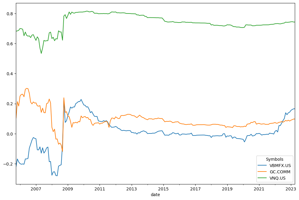
Sometimes it’s better to verify the rolling correlation with the benchmark (S&P 500 Total Return index).

Rolling period size is set with rolling_window attribute in months.

[16]:

x.index_corr(rolling_window=12 * 5).plot();  # rolling window size is 5 years

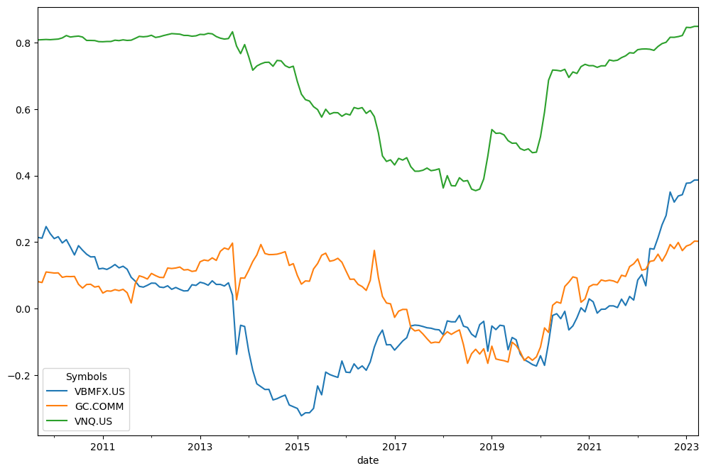
It can be clearly seen that real estat ETF (VNQ) has higher correlation with stocks comparing with gold prices and bonds during this period.

[ ]: