EfficientFrontier
- class EfficientFrontier(assets=None, *, first_date=None, last_date=None, ccy='USD', bounds=None, inflation=False, full_frontier=True, rebalancing_strategy=period year abs_deviation NaN rel_deviation NaN dtype: str, n_points=20, verbose=False, ticker_names=True)
Bases:
AssetListEfficient Frontier with multi-period optimization.
In multi-period optimization, portfolios are rebalanced according to a rebalancing strategy.
Rebalancing is the process by which an investor restores a portfolio to its target allocation by selling and buying assets. After rebalancing, the portfolio assets have their target weights.
- Parameters:
- assetslist[str]
List of assets. Could include tickers or asset-like objects (Asset, Portfolio). Must contain at least two assets.
- first_datestr, default None
First date of monthly return time series. If None the first date is calculated automatically as the oldest available date for the listed assets.
- last_datestr, default None
Last date of monthly return time series. If None the last date is calculated automatically as the newest available date for the listed assets.
- ccystr, default ‘USD’
Base currency for the list of assets. All risk metrics and returns are adjusted to the base currency.
- boundstuple[tuple[float, float], …] or None, default None
Bounds for asset weights. Each asset weight is constrained within the corresponding (min, max) pair. For example, ((0.0, 0.5), (0.0, 1.0)) restricts the first asset to [0%, 50%] and leaves the second asset unconstrained.
- inflationbool, default False
Defines whether to take inflation data into account in the calculations. Including inflation could limit available data (first_date, last_date) as the inflation data is usually published with a one-month delay.
- rebalancing_strategyRebalance, default Rebalance(period=’year’)
Rebalancing strategy used to generate portfolio return series during optimization. Only rebalancing_strategy.period is used; abs_deviation and rel_deviation are ignored.
- n_pointsint, default 20
Number of points in the Efficient Frontier.
- full_frontierbool, default True
Defines whether to show the full Efficient Frontier or only its upper part. If ‘False’ Efficient Frontier has only the points with the return above Global Minimum Volatility (GMV) point.
- verbosebool, default False
If verbose=True calculates elapsed time for each point and the total elapsed time.
- ticker_namesbool, default True
Defines whether to include full names of assets in the optimization report or only tickers.
Notes
For classic single-period (monthly rebalanced, constant-weight) optimization, use EfficientFrontierSingle.
Methods & Attributes
Return bounds for the assets weights.
Generate multi-period Efficient Frontier.
get_grid_portfolios([step, max_points])Generate rebalanced portfolios for all weight combinations on a grid.
get_monte_carlo([n])Generate random rebalanced portfolios with Monte Carlo simulation.
get_most_diversified_portfolio([target_return])Calculate assets weights and portfolio metrics for the most diversified portfolio within bounds.
get_tangency_portfolio([rf_return, ...])Calculate asset weights, risk and return values for tangency portfolio within given bounds.
Find a portfolio with global max CAGR.
Calculate the annualized risk (standard deviation) and CAGR of the Global Minimum Volatility portfolio.
Calculate asset weights of the Global Minimum Volatility (GMV) portfolio.
Calculate asset weights of the Global Minimum Volatility (GMV) portfolio.
Label mode for reports/charts: 'ticker', 'name' or 'local_name'.
Generate Most diversified portfolios frontier for rebalanced portfolios.
minimize_risk(target_value)Calculate the portfolio properties to minimize annualized risk at the target CAGR.
Return or set number of points in the Efficient Frontier.
plot_cml([rf_return, figsize])Plot Capital Market Line (CML).
plot_pair_ef([tickers, figsize])Plot Efficient Frontier for every pair of assets.
plot_transition_map([x_axe, figsize])Plot Transition Map for optimized portfolios on the Efficient Frontier.
Rebalancing strategy used to compute portfolio return series during optimization.
Calculate range of annualized risk values (from min risk to max risk).
Legacy flag: True shows tickers, False shows full names.
Return or set whether to show technical information during the optimization.
- property bounds
Return bounds for the assets weights.
Bounds are used in optimization. Each asset can have weights limitation from 0 to 1.0.
If an asset has limitation for 10 to 20% bounds are defined as (0.1, 0.2). bounds = ((0, .5), (0, 1)) shows that in Portfolio with two assets first one has weight limitations from 0 to 50%. The second asset has no limitations.
- Returns:
- tuple of ((float, float),…)
Weights bounds used for portfolio optimization.
Examples
>>> two_assets = ok.EfficientFrontierSingle(["SPY.US", "AGG.US"])
>>> two_assets.bounds
((0.0, 1.0), (0.0, 1.0))
By default there are no limitations for assets weights. Bounds can be set for a Efficient Frontier object.
>>> two_assets.bounds = ((0.5, 0.9), (0, 1.0))
Now the optimization is bounded (SPY has weights limits from 50 to 90%).
- property n_points
Return or set number of points in the Efficient Frontier.
- Returns:
- int
Number of points in the Efficient Frontier.
Examples
>>> frontier = ok.EfficientFrontier(["SPY.US", "BND.US"])
>>> frontier.n_points  # default number of points
20
- property rebalancing_strategy
Rebalancing strategy used to compute portfolio return series during optimization.
Only rebalancing_strategy.period is used in the optimization; abs_deviation and rel_deviation are ignored.
- Returns:
- Rebalance
Rebalancing strategy.
Examples
>>> frontier = ok.EfficientFrontier(["SPY.US", "BND.US"])
>>> frontier.rebalancing_strategy.period
'year'
>>> frontier.rebalancing_strategy = ok.Rebalance(period="none")
- property ticker_names
Legacy flag: True shows tickers, False shows full names.
- property labels
Label mode for reports/charts: ‘ticker’, ‘name’ or ‘local_name’.
- property verbose
Return or set whether to show technical information during the optimization.
- Returns:
- bool
- get_most_diversified_portfolio(target_return=None)
Calculate assets weights and portfolio metrics for the most diversified portfolio within bounds.
The most diversified portfolio is defined as the portfolio with the maximum Diversification Ratio.
- Parameters:
- target_returnfloat, default None
Target Compound Annual Growth Rate (CAGR) for the portfolio. If provided, the optimizer searches for a portfolio with the target CAGR and the maximum Diversification Ratio. If None, the global most diversified portfolio is returned.
- Returns:
- dict[str, float]
Mapping with asset weights (keys are tickers or asset names depending on ticker_names) and portfolio metrics: ‘CAGR’, ‘Risk’, and ‘Diversification ratio’.
Examples
>>> ls4 = ["SPY.US", "AGG.US", "VNQ.US", "GLD.US"]
>>> x = ok.EfficientFrontier(assets=ls4, ccy="USD", last_date="2021-12")
>>> x.get_most_diversified_portfolio()  # get a global most diversified portfolio
{'SPY.US': 0.19612726258395477,
'AGG.US': 0.649730553241489,
'VNQ.US': 0.020096313783052246,
'GLD.US': 0.13404587039150392,
'CAGR': 0.062355715886719176,
'Risk': 0.05510135025563423,
'Diversification ratio': 1.5665720501693001}
It is possible to get the most diversified portfolio for a given target CAGR.
>>> x.get_most_diversified_portfolio(target_return=0.10)
{'SPY.US': 0.3389762570274293,
'AGG.US': 0.12915657041748244,
'VNQ.US': 0.15083042115027034,
'GLD.US': 0.3810367514048179,
'CAGR': 0.09370688842211439,
'Risk': 0.11725067815643951,
'Diversification ratio': 1.4419864802150442}
- get_tangency_portfolio(rf_return=0, rate_of_return='cagr')
Calculate asset weights, risk and return values for tangency portfolio within given bounds.
Tangency portfolio or Maximum Sharpe Ratio (MSR) is the point on the Efficient Frontier where Sharpe Ratio reaches its maximum.
The Sharpe ratio is the average annual return in excess of the risk-free rate per unit of risk (annualized standard deviation).
Bounds are defined with ‘bounds’ property.
- Parameters:
- rf_returnfloat, default 0
Risk-free rate of return.
- rate_of_return{‘cagr’, ‘mean_return’}, default ‘cagr’
Return definition used to calculate Sharpe ratio.
‘cagr’: Compound Annual Growth Rate.
‘mean_return’: Arithmetic mean return (annualized).
- Returns:
- dict
Weights of assets, risk and return of the tangency portfolio.
Examples
>>> three_assets = ["SPY.US", "AGG.US", "GLD.US"]
>>> ef = ok.EfficientFrontier(assets=three_assets, ccy="USD", last_date="2022-06")
>>> msr = ef.get_tangency_portfolio(rf_return=0.03)  # risk free rate of return is 3%
>>> msr
{'Weights': array([0.47687653, 0.25779952, 0.26532395]),
'Rate_of_return': 0.07759168028010821,
'Risk': 0.0959884843475395}
To calculate tangency portfolio parameters for arithmetic mean set rate_of_return=’mean_return’:
>>> msr_mean = ef.get_tangency_portfolio(rate_of_return="mean_return", rf_return=0.03)
>>> msr_mean
{'Weights': array([0.61143897, 0.00159518, 0.38696585]),
'Rate_of_return': 0.09876868143927053,
'Risk': 0.12609086541280776}
- property gmv_monthly_weights
Calculate asset weights of the Global Minimum Volatility (GMV) portfolio. The objective function is monthly risk (standard deviation of return).
Global Minimum Volatility portfolio is a portfolio with the lowest risk of all possible. Along the Efficient Frontier, the left-most point is a portfolio with minimum risk when compared to all possible portfolios of risky assets.
- Returns:
- numpy.ndarray
GMV portfolio assets weights.
Examples
>>> frontier = ok.EfficientFrontier(["SPY.US", "AGG.US"])
>>> frontier.gmv_monthly_weights
array([0.0578446, 0.9421554])
- property gmv_annual_weights
Calculate asset weights of the Global Minimum Volatility (GMV) portfolio. The objective function is annualized risk (standard deviation of return).
Global Minimum Volatility portfolio is a portfolio with the lowest risk of all possible. Along the Efficient Frontier, the left-most point is a portfolio with minimum risk when compared to all possible portfolios of risky assets.
- Returns:
- numpy.ndarray
GMV portfolio assets weights.
Examples
>>> frontier = ok.EfficientFrontier(["SPY.US", "AGG.US"])
>>> frontier.gmv_monthly_weights
array([0.05373824, 0.94626176])
- property gmv_annual_values
Calculate the annualized risk (standard deviation) and CAGR of the Global Minimum Volatility portfolio.
Global Minimum Volatility portfolio is a portfolio with the lowest risk of all possible. Compound annual growth rate (CAGR) is the rate of return that would be required for an investment to grow from its initial to its final value, assuming all incomes were reinvested.
- Returns:
- tuple
Annualized value of risk (standard deviation), Compound annual growth rate (CAGR) for Global Minimum Volatility portfolio (GMV).
Examples
>>> frontier = ok.EfficientFrontier(["SPY.US", "AGG.US"])
>>> frontier.gmv_annual_values
(0.03695845106087943, 0.04418318557516887)
- property global_max_return_portfolio
Find a portfolio with global max CAGR.
Compound annual growth rate (CAGR) is the rate of return that would be required for an investment to grow from its initial to its final value, assuming all incomes were reinvested.
The objective function is Accumulated return for rebalanced portfolio time series for the period from ‘first_date’ to ‘last_date’.
- Returns:
- dict
Weights of assets, CAGR, annualized risk, monthly risk.
Examples
>>> frontier = ok.EfficientFrontier(["SPY.US", "AGG.US"])
>>> frontier.global_max_return_portfolio
{'Weights': array([1., 0.]), 'CAGR': 0.10797159166196812, 'Risk': 0.1583011735798155, 'Risk_monthly': 0.0410282468594492}
- minimize_risk(target_value)
Calculate the portfolio properties to minimize annualized risk at the target CAGR.
This method finds the portfolio weights that minimize the annualized risk (standard deviation) while achieving a specified target Compound Annual Growth Rate (CAGR).
The optimization is performed for a rebalanced portfolio over the period from ‘first_date’ to ‘last_date’. CAGR is the rate of return required for an investment to grow from its initial to its final value, assuming all incomes were reinvested.
- Parameters:
- target_valuefloat
Target Compound Annual Growth Rate (CAGR) for the portfolio. Should be a decimal value (e.g., 0.107 for 10.7% annual return).
- Returns:
- dict
Dictionary containing: - Asset weights (one key per asset symbol or name) - ‘CAGR’: Target CAGR value - ‘Risk’: Minimized annualized risk (standard deviation) - ‘Weights’: Array of optimal weights - ‘iterations’: Number of optimization iterations performed
- Raises:
- RuntimeError
If no solution is found for the given target CAGR value.
Examples
>>> frontier = ok.EfficientFrontier(["SPY.US", "AGG.US"])
>>> point = frontier.minimize_risk(0.08)
>>> round(point["CAGR"], 2)
0.08
- property annual_return_ts
Calculate annual rate of return time series for each asset.
Rate of return is calculated for each calendar year.
- Returns:
- DataFrame
Calendar annual rate of return time series.
Examples
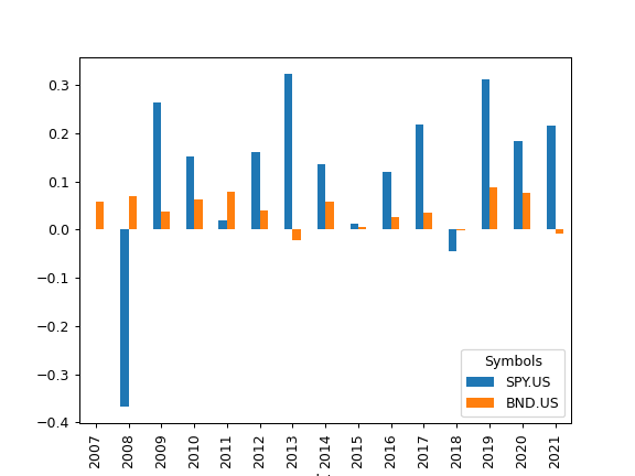
>>> import matplotlib.pyplot as plt
>>> al = ok.AssetList(["SPY.US", "BND.US"], last_date="2021-08")
>>> al.annual_return_ts.plot(kind="bar")
>>> plt.show()
- property assets_close_monthly
Show assets monthly close time series adjusted to the base currency.
- Returns:
- DataFrame
Assets monthly close time series adjusted to the base currency.
Examples
>>> import matplotlib.pyplot as plt
>>> al = ok.AssetList(["SPY.US", "BND.US"], ccy="USD")
>>> al.assets_close_monthly.plot()
>>> plt.show()
- property assets_ror
Rate of return monthly time series for all assets.
- Returns:
- DataFrame
Rate of return monthly data.
- property currency
Return the base currency.
Such properties as rate of return and risk are adjusted to the base currency.
- Returns:
- str
Base currency.
- describe(years=(1, 5, 10), tickers=True)
Generate descriptive statistics for a list of assets.
Statistics includes:
YTD (Year To date) compound return
CAGR for a given list of periods and full available period
Annualized mean rate of return (full available period)
LTM Dividend yield - last twelve months dividend yield
Risk metrics (full period):
risk (standard deviation)
CVAR (timeframe is 1 year)
max drawdowns (and dates of the drawdowns)
Statistics also shows for each asset: - inception date - first date available for each asset - last asset date - available for each asset date - Common last data date - common for the asset list data (may be set by last_date manually)
- Parameters:
- yearstuple of int, default (1, 5, 10)
List of periods for CAGR.
- tickersbool or str, default True
Defines which labels to use in the column header. A bool value uses tickers (True) or asset names (False) for legacy compatibility. A string value selects the mode explicitly: ‘tickers’, ‘names’, or ‘local_names’.
- Returns:
- DataFrame
Table of descriptive statistics for a list of assets.
See also
get_cumulative_returnCalculate cumulative return.
get_cagrCalculate assets Compound Annual Growth Rate (CAGR).
dividend_yieldCalculate dividend yield (LTM).
risk_annualReturn annualized risks (standard deviation).
get_cvar_historicCalculate historic Conditional Value at Risk (CVaR).
drawdownsCalculate drawdowns.
Examples
>>> al = ok.AssetList(["SPY.US", "AGG.US"], last_date="2021-08")
>>> al.describe(years=[1, 10, 15])
                 property               period    AGG.US    SPY.US inflation
0         Compound return                  YTD -0.005620  0.180519  0.048154
1                    CAGR              1 years -0.007530  0.363021  0.053717
2                    CAGR             10 years  0.032918  0.152310  0.019136
3                    CAGR             15 years  0.043013  0.107598  0.019788
4                    CAGR  17 years, 10 months  0.039793  0.107972  0.022002
5          Dividend yield                  LTM  0.018690  0.012709       NaN
6                    Risk  17 years, 10 months  0.037796  0.158301       NaN
7                    CVAR  17 years, 10 months  0.023107  0.399398       NaN
- property dividend_growing_years
Return the number of years when the annual dividend was growing for each asset.
- Returns:
- DataFrame
Dividend growth length periods time series for each asset.
See also
dividend_yieldDividend yield time series.
dividend_yield_annualCalendar year dividend yield time series.
dividends_annualCalendar year dividends.
dividend_paying_yearsNumber of years of consecutive dividend payments.
get_dividend_mean_yieldArithmetic mean for annual dividend yield.
get_dividend_mean_growth_rateGeometric mean of annual dividends growth rate.
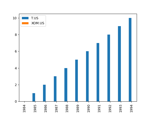
Examples
>>> import matplotlib.pyplot as plt
>>> x = ok.AssetList(["T.US", "XOM.US"], first_date="1984-01", last_date="1994-12")
>>> x.dividend_growing_years.plot(kind="bar")
>>> plt.show()
- property dividend_paying_years
Return the number of years of consecutive dividend payments for each asset.
- Returns:
- DataFrame
Dividend payment period length time series for each asset.
See also
dividend_yieldDividend yield time series.
dividend_yield_annualCalendar year dividend yield time series.
dividends_annualCalendar year dividends.
dividend_growing_yearsNumber of years when the annual dividend was growing.
get_dividend_mean_yieldArithmetic mean for annual dividend yield.
get_dividend_mean_growth_rateGeometric mean of annual dividends growth rate.
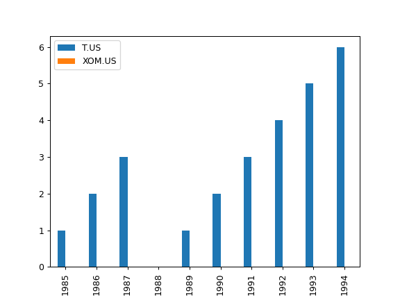
Examples
>>> import matplotlib.pyplot as plt
>>> x = ok.AssetList(["T.US", "XOM.US"], first_date="1984-01", last_date="1994-12")
>>> x.dividend_paying_years.plot(kind="bar")
>>> plt.show()
- property dividend_yield
Calculate last twelve months (LTM) dividend yield time series (monthly) for each asset.
LTM dividend yield is the sum trailing twelve months of common dividends per share divided by the current price per share.
All yields are calculated in the asset list base currency after adjusting the dividends and price time series. Forecasted (future) dividends are removed. Zero value time series are created for assets without dividends.
- Returns:
- DataFrame
Time series of LTM dividend yield for each asset.
See also
dividend_yield_annualCalendar year dividend yield time series.
dividends_annualCalendar year dividends time series.
dividend_paying_yearsNumber of years of consecutive dividend payments.
dividend_growing_yearsNumber of years when the annual dividend was growing.
get_dividend_mean_yieldArithmetic mean for annual dividend yield.
get_dividend_mean_growth_rateGeometric mean of annual dividends growth rate.
Examples
>>> x = ok.AssetList(["T.US", "XOM.US"], first_date="1984-01", last_date="1994-12")
>>> x.dividend_yield
           T.US    XOM.US
1984-01  0.000000  0.000000
1984-02  0.000000  0.002597
1984-03  0.002038  0.002589
1984-04  0.001961  0.002346
           ...       ...
1994-09  0.018165  0.012522
1994-10  0.018651  0.011451
1994-11  0.018876  0.012050
1994-12  0.019344  0.011975
[132 rows x 2 columns]
- property dividend_yield_annual
Calculate last twelve months (LTM) dividend yield annual time series.
Time series is based on the dividend yield for the end of calendar year.
LTM dividend yield is the sum trailing twelve months of common dividends per share divided by the current price per share.
All yields are calculated in the asset list base currency after adjusting the dividends and price time series. Forecasted (future) dividends are removed.
- Returns:
- DataFrame
Time series of LTM dividend yield for each asset.
See also
dividend_yieldDividend yield time series.
dividends_annualCalendar year dividends time series.
dividend_paying_yearsNumber of years of consecutive dividend payments.
dividend_growing_yearsNumber of years when the annual dividend was growing.
get_dividend_mean_yieldArithmetic mean for annual dividend yield.
get_dividend_mean_growth_rateGeometric mean of annual dividends growth rate.
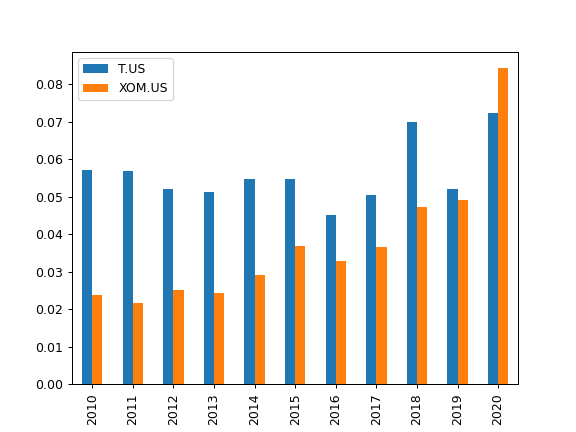
Examples
>>> import matplotlib.pyplot as plt
>>> x = ok.AssetList(["T.US", "XOM.US"], first_date="2010-01", last_date="2020-12")
>>> x.dividend_yield_annual.plot(kind="bar")
>>> plt.show()
- property dividends_annual
Return calendar year dividends sum time series for each asset.
- Returns:
- DataFrame
Annual dividends time series for each asset.
See also
dividend_yieldDividend yield time series.
dividend_yield_annualCalendar year dividend yield time series.
dividend_paying_yearsNumber of years of consecutive dividend payments.
dividend_growing_yearsNumber of years when the annual dividend was growing.
get_dividend_mean_yieldArithmetic mean for annual dividend yield.
get_dividend_mean_growth_rateGeometric mean of annual dividends growth rate.
Examples
>>> import matplotlib.pyplot as plt
>>> x = ok.AssetList(["T.US", "XOM.US"], first_date="2010-01", last_date="2020-12")
>>> x.dividends_annual.plot(kind="bar")
>>> plt.show()
- property drawdowns
Calculate drawdowns time series for the assets.
The drawdown is the percent decline from a previous peak in wealth index.
- Returns:
- DataFrame
Time series of drawdowns.
See also
risk_monthlyCalculate montly risk for each asset.
risk_annualCalculate annualized risks.
semideviation_monthlyCalculate semideviation monthly values.
semideviation_annualCalculate semideviation annualized values.
get_var_historicCalculate historic Value at Risk (VaR).
get_cvar_historicCalculate historic Conditional Value at Risk (CVaR).
Examples
>>> import matplotlib.pyplot as plt
>>> al = ok.AssetList(["SPY.US", "BND.US"], last_date="2021-08")
>>> al.drawdowns.plot()
>>> plt.show()
- get_cagr(period=None, real=False)
Calculate the expanding Compound Annual Growth Rate (CAGR) time series for each asset.
The expanding CAGR at each month is the annualized rate of return required for the investment to grow from its initial value to its value at that month, assuming all incomes were reinvested. The last row contains the CAGR over the full selected period.
Inflation adjusted annualized returns (real CAGR) are shown with real=True option. Annualized inflation is calculated for the same period if inflation=True in the AssetList.
- Parameters:
- periodint, default None
CAGR trailing period in years. If None, use the full available period.
- realbool, default False
CAGR is adjusted for inflation (real CAGR) if True. AssetList should be initiated with inflation=True for real CAGR.
- Returns:
- DataFrame
Time series of expanding CAGR for each asset and annualized inflation (if inflation=True in AssetList and real=False).
See also
get_rolling_cagrCalculate rolling CAGR.
get_cumulative_returnCalculate expanding cumulative return.
Notes
CAGR is not defined for periods less than 1 year. The first 11 rows are filled with NaN values.
Examples
>>> x = ok.AssetList(["SPY.US"], ccy="USD", inflation=True)
>>> x.get_cagr(period=5).tail()
           SPY.US  USD.INFL
2024-08  0.137419  0.030126
2024-09  0.144211  0.031120
2024-10  0.150951  0.032150
2024-11  0.146517  0.031044
2024-12  0.151012  0.029504
The last row contains the CAGR values over the full selected period.
To get inflation adjusted annualized return (real CAGR) add real=True option:
>>> x = ok.AssetList(["EURUSD.FX", "CNYUSD.FX"], inflation=True)
>>> x.get_cagr(period=5, real=True).tail()
- get_cumulative_return(period=None, real=False)
Calculate the expanding cumulative return time series for each asset.
The cumulative return is the total compounded change in the asset price from the start of the selected period up to and including each subsequent month. The last row contains the cumulative return over the full selected period.
Inflation adjusted cumulative returns (real cumulative returns) are shown with real=True option. Inflation data is taken from the same period if inflation=True in the AssetList.
- Parameters:
- periodstr or int or None, default None
Trailing period in years. Period should be greater than 0. None - full time cumulative return. ‘YTD’ - (Year To Date) period of time beginning the first day of the calendar year up to the last month.
- realbool, default False
Cumulative return is adjusted for inflation (real cumulative return) if True. AssetList should be initiated with inflation=True for real cumulative return.
- Returns:
- DataFrame
Time series of cumulative return for each asset and cumulative inflation (if inflation=True in AssetList and real=False).
See also
get_rolling_cagrCalculate rolling CAGR.
get_cagrCalculate CAGR.
get_rolling_cumulative_returnCalculate rolling cumulative return.
annual_returnCalculate annualized mean return (arithmetic mean).
Examples
>>> x = ok.AssetList(["MCFTR.INDX"], ccy="RUB")
>>> x.get_cumulative_return(period="YTD").tail()
         MCFTR.INDX  RUB.INFL
2024-08    0.083117  0.031241
2024-09    0.094772  0.035987
2024-10    0.118014  0.042601
2024-11    0.131562  0.046832
2024-12    0.148300  0.048500
The last row contains the YTD cumulative return values.
- get_cvar_historic(time_frame=12, level=1)
Calculate historic Conditional Value at Risk (CVAR, expected shortfall) for the assets with a given timeframe.
CVaR is the average loss over a specified time period of unlikely scenarios beyond the confidence level. Loss is a positive number (expressed in cumulative return). If CVaR is negative there are expected gains at this confidence level.
- Parameters:
- time_frameint, default 12
Time period size in months
- levelint, default 1
Confidence level in percents to calculate the VaR. Default value is 1% (1% quantile).
- Returns:
- Series
CVaR values for each asset in form of Series.
See also
risk_monthlyCalculate montly risk for each asset.
risk_annualCalculate annualized risks.
semideviation_monthlyCalculate semideviation monthly values.
semideviation_annualCalculate semideviation annualized values.
get_var_historicCalculate historic Value at Risk (VaR).
drawdownsCalculate drawdowns.
Examples
>>> x = ok.AssetList(["SPY.US", "AGG.US"])
>>> x.get_cvar_historic(time_frame=60, level=1)
SPY.US    0.2574
AGG.US   -0.0766
dtype: float64
Name: VaR, dtype: float64
- get_dividend_mean_growth_rate(period=5)
Calculate geometric mean of annual dividends growth rate time series for a given trailing period.
Growth rate is taken for full calendar annual dividends.
- Parameters:
- periodint, default 5
Growth rate trailing period in years. Period should be a positive integer and not exceed the available data period_length.
- Returns:
- Series
Dividend growth geometric mean value for each asset.
See also
dividend_yieldDividend yield time series.
dividend_yield_annualCalendar year dividend yield time series.
dividends_annualCalendar year dividends.
dividend_paying_yearsNumber of years of consecutive dividend payments.
dividend_growing_yearsNumber of years when the annual dividend was growing.
get_dividend_mean_yieldArithmetic mean for annual dividend yield.
Examples
>>> x = ok.AssetList(["T.US", "XOM.US"], first_date="1984-01", last_date="1994-12")
>>> x.get_dividend_mean_growth_rate(period=3)
T.US      0.020067
XOM.US    0.024281
dtype: float64
- get_dividend_mean_yield(period=5)
Calculate the arithmetic mean for annual dividend yield (LTM) over a specified period.
Dividend yield is taken for full calendar annual dividends.
- Parameters:
- periodint, default 5
Mean dividend yield trailing period in years. Period should be a positive integer and not exceed the available data period_length.
- Returns:
- Series
Mean dividend yield value for each asset.
See also
dividend_yieldDividend yield time series.
dividend_yield_annualCalendar year dividend yield time series.
dividends_annualCalendar year dividends.
get_dividend_mean_growth_rateGeometric mean of annual dividends growth rate.
dividend_paying_yearsNumber of years of consecutive dividend payments.
dividend_growing_yearsNumber of years when the annual dividend was growing.
Examples
>>> al = ok.AssetList(["SBERP.MOEX", "LKOH.MOEX"], ccy="RUB", first_date="2005-01", last_date="2023-12")
>>> al.get_dividend_mean_yield(period=3)
SBERP.MOEX    0.052987
LKOH.MOEX     0.156526
dtype: float64
- get_monthly_geometric_mean_return()
Calculate monthly geometric mean return for each asset.
The geometric mean return is the constant periodic return that would produce the same final value as a sequence of varying periodic returns when compounded over time.
- Returns:
- Series
Monthly geometric mean return value for each asset.
Examples
>>> al = ok.AssetList(["SPY.US", "AGG.US"])
>>> al.get_monthly_geometric_mean_return()
SPY.US    0.008456
AGG.US    0.003124
dtype: float64
- get_rolling_cagr(window=12, real=False)
Calculate rolling CAGR for each asset.
Compound annual growth rate (CAGR) is the rate of return that would be required for an investment to grow from its initial to its final value, assuming all incomes were reinvested.
Inflation adjusted annualized returns (real CAGR) are shown with real=True option.
- Parameters:
- windowint, default 12
Size of the moving window in months. Window size should be at least 12 months for CAGR.
- realbool, default False
CAGR is adjusted for inflation (real CAGR) if True. AssetList should be initiated with inflation=True for real CAGR.
- Returns:
- DataFrame
Time series of rolling CAGR and mean inflation (optionally).
See also
get_rolling_cagrCalculate rolling CAGR.
get_cagrCalculate CAGR.
get_rolling_cumulative_returnCalculate rolling cumulative return.
annual_returnCalculate annualized mean return (arithmetic mean).
Notes
CAGR is not defined for periods less than 1 year (NaN values are returned).
Examples
>>> import matplotlib.pyplot as plt
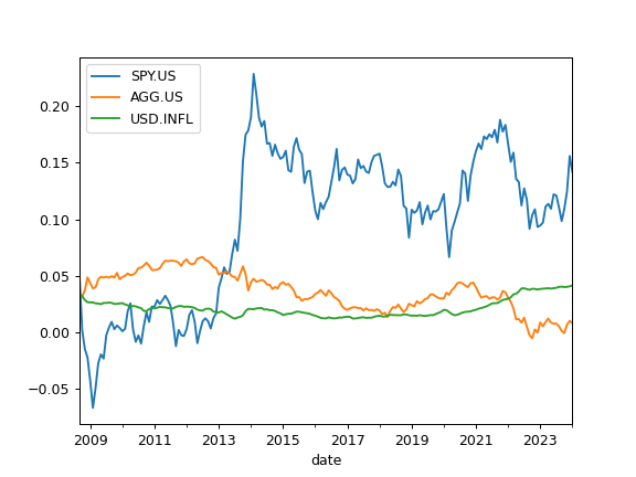
>>> x = ok.AssetList(["SPY.US", "AGG.US"], ccy="USD", inflation=True)
>>> x.get_rolling_cagr(window=5 * 12).plot()
>>> plt.show()
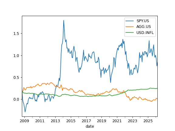
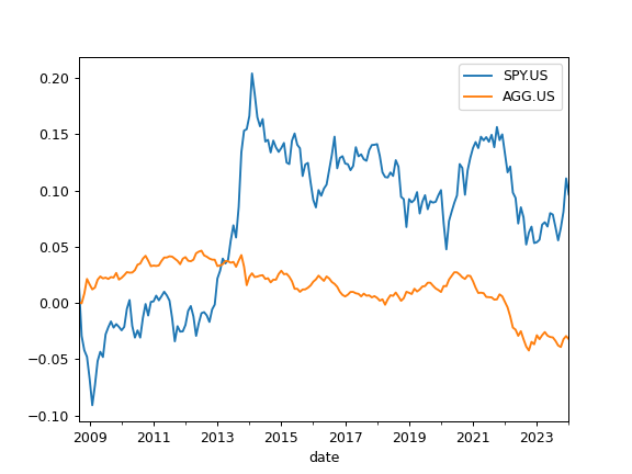
For inflation adjusted rolling CAGR add ‘real=True’ option:
>>> x.get_rolling_cagr(window=5 * 12, real=True).plot()
>>> plt.show()
- get_rolling_cumulative_return(window=12, real=False)
Calculate rolling cumulative return for each asset.
The cumulative return is the total change in the asset price.
- Parameters:
- windowint, default 12
Size of the moving window in months.
- realbool, default False
Cumulative return is adjusted for inflation (real cumulative return) if True. AssetList should be initiated with inflation=True for real cumulative return.
- Returns:
- DataFrame
Time series of rolling cumulative return.
See also
get_rolling_cagrCalculate rolling CAGR.
get_cagrCalculate CAGR.
get_cumulative_returnCalculate cumulative return.
annual_returnCalculate annualized mean return (arithmetic mean).
Examples
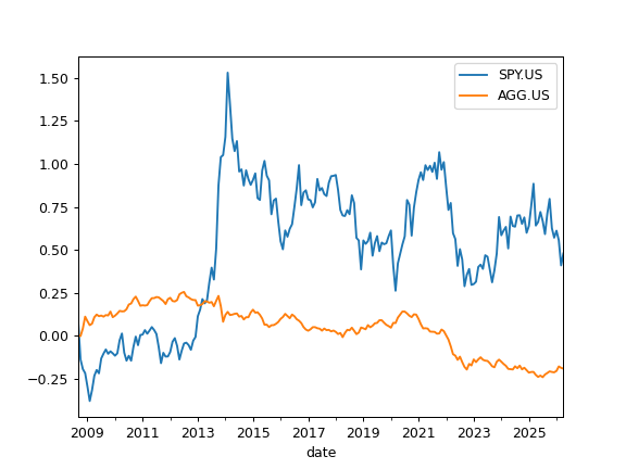
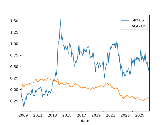
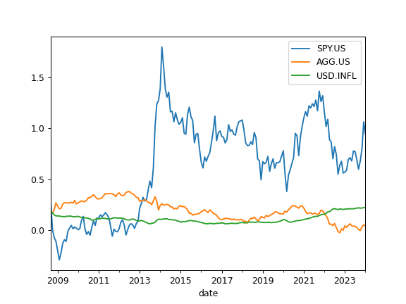
>>> import matplotlib.pyplot as plt
>>> x = ok.AssetList(["SPY.US", "AGG.US"], ccy="USD", inflation=True)
>>> x.get_rolling_cumulative_return(window=5 * 12).plot()
>>> plt.show()

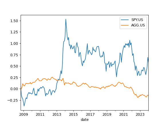
For inflation adjusted rolling cumulative return add ‘real=True’ option:
>>> x.get_rolling_cumulative_return(window=5 * 12, real=True).plot()
>>> plt.show()
- get_rolling_risk_annual(window=12)
Calculate annualized risk rolling time series for each asset.
Risk is a standard deviation of the rate of return.
Annualized risk time series is calculated for the rate of return values limited by moving window.
- Parameters:
- windowint, default 12
Size of the moving window in months.
- Returns:
- DataFrame
Annualized risk (standard deviation) rolling time series for each asset.
See also
risk_monthlyCalculate montly risk expanding time series for each asset.
risk_annualCalculate annualized risks.
semideviation_monthlyCalculate semideviation monthly values.
semideviation_annualCalculate semideviation annualized values.
get_var_historicCalculate historic Value at Risk (VaR).
get_cvar_historicCalculate historic Conditional Value at Risk (CVaR).
drawdownsCalculate assets drawdowns.
Examples
>>> import matplotlib.pyplot as plt
>>> x = ok.AssetList(["SPY.US", "AGG.US"], ccy="USD", inflation=True)
>>> x.get_rolling_risk_annual(window=5 * 12).plot()
>>> plt.show()
- get_sharpe_ratio(rf_return=0)
Calculate Sharpe ratio for the assets.
The Sharpe ratio is the average annual return in excess of the risk-free rate per unit of risk (annualized standard deviation).
Risk-free rate should be taken according to the AssetList base currency.
- Parameters:
- rf_returnfloat, default 0
Risk-free rate of return.
- Returns:
- pd.Series
Examples
>>> al = ok.AssetList(["VOO.US", "BND.US"])
>>> al.get_sharpe_ratio(rf_return=0.02)
VOO.US    0.962619
BND.US    0.390814
dtype: float64
- get_sortino_ratio(t_return=0)
Calculate Sortino ratio for the assets with specified target return.
Sortion ratio measures the risk-adjusted return of each asset. It is a modification of the Sharpe ratio but penalizes only those returns falling below a specified target rate of return, while the Sharpe ratio penalizes both upside and downside volatility equally.
- Parameters:
- t_returnfloat, default 0
Traget rate of return.
- Returns:
- pd.Series
Examples
>>> al = ok.AssetList(["VOO.US", "BND.US"], last_date="2021-12")
>>> al.get_sortino_ratio(t_return=0.03)
VOO.US    1.321951
BND.US    0.028969
dtype: float64
- get_var_historic(time_frame=12, level=1)
Calculate historic Value at Risk (VaR) for the assets with a given timeframe.
The VaR calculates the potential loss of an investment with a given time frame and confidence level. Loss is a positive number (expressed in cumulative return). If VaR is negative there are expected gains at this confidence level.
- Parameters:
- time_frameint, default 12
Time period size in months
- levelint, default 1
Confidence level in percents (1 - 100%). Default value is 1%.
- Returns:
- Series
VaR values for each asset in form of Series.
See also
risk_monthlyCalculate montly risk for each asset.
risk_annualCalculate annualized risks.
semideviation_monthlyCalculate semideviation monthly values.
semideviation_annualCalculate semideviation annualized values.
get_cvar_historicCalculate historic Conditional Value at Risk (CVaR).
drawdownsCalculate drawdowns.
Examples
>>> x = ok.AssetList(["SPY.US", "AGG.US"])
>>> x.get_var_historic(time_frame=60, level=1)
SPY.US    0.2101
AGG.US    -0.0867
Name: VaR, dtype: float64
- index_beta(rolling_window=None)
Compute beta coefficient time series for the assets.
Beta coefficient is defined in Capital Asset Pricing Model (CAPM). It is a measure of how an individual asset moves (on average) when the benchmark increases or decreases. When beta is positive, the asset price tends to move in the same direction as the benchmark, and the magnitude of beta tells by how much.
Index (benchmark) should be in the first position of the symbols list in AssetList parameters. There should be at least 12 months of historical data.
- Parameters:
- rolling_windowint or None, default None
Size of the moving window in months. Must be at least 12 months. If None calculate expanding beta coefficient.
- Returns:
- DataFrame
rollinf or expanding beta coefficient time series for each asset.
See also
index_corrCompute correlation with the index (or benchmark).
index_rolling_corrCompute rolling correlation with the index (or benchmark).
index_betaCompute beta coefficient.
Examples
>>> import matplotlib.pyplot as plt
>>> sp = ok.AssetList(["SP500TR.INDX", "VBMFX.US", "GC.COMM", "VNQ.US"])
>>> sp.names
{'SP500TR.INDX': 'S&P 500 (TR)',
'VBMFX.US': 'VANGUARD TOTAL BOND MARKET INDEX FUND INVESTOR SHARES',
'GC.COMM': 'Gold',
'VNQ.US': 'Vanguard Real Estate Index Fund ETF Shares'}
>>> sp.index_beta().plot()
>>> plt.show()
To calculate rolling beta set rolling_window to a number of months (moving window size):
>>> sp.index_beta(rolling_window=12 * 5).plot()  # 5 years moving window
>>> plt.show()
- index_corr(rolling_window=None)
Compute correlation with the index (or benchmark) time series for the assets. Expanding or rolling correlation is available.
Index (benchmark) should be in the first position of the symbols list in AssetList parameters. There should be at least 12 months of historical data.
- Parameters:
- rolling_windowint or None, default None
Size of the moving window in months. Must be at least 12 months. If None calculate expanding correlation with index.
- Returns:
- DataFrame
Rolling or expanding correlation with the index (or benchmark) time series for each asset.
Examples
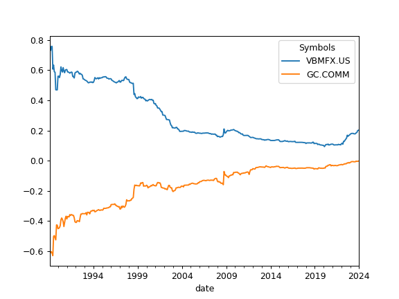
>>> import matplotlib.pyplot as plt
>>> sp = ok.AssetList(["SP500TR.INDX", "VBMFX.US", "GC.COMM"])
>>> sp.names
{'SP500TR.INDX': 'S&P 500 (TR)',
'VBMFX.US': 'VANGUARD TOTAL BOND MARKET INDEX FUND INVESTOR SHARES',
'GC.COMM': 'Gold'}
>>> sp.index_corr().plot()  # expanding correlation with S&P 500
>>> plt.show()
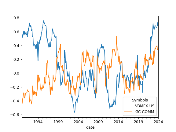
To calculate rolling correlation with S&P 500 set rolling_window to a number of months (moving window size):
>>> sp.index_corr(rolling_window=24).plot()
>>> plt.show()
- property jarque_bera
Perform Jarque-Bera test for normality of assets returns historical data.
Jarque-Bera test shows whether the returns have the skewness and kurtosis matching a normal distribution (null hypothesis or H0).
- Returns:
- DataFrame
Returns test statistic and the p-value for the hypothesis test. Large Jarque-Bera statistics and tiny p-value (< 0.05) indicate that null hypothesis (H0) is rejected and the time series is not normally distributed. Low statistic numbers correspond to normal distribution.
See also
skewnessCompute skewness.
skewness_rollingCompute rolling skewness.
kurtosisCalculate expanding Fisher (normalized) kurtosis.
kurtosis_rollingCalculate rolling Fisher (normalized) kurtosis.
kstestPerform Kolmogorov-Smirnov test for different types of distributions.
Examples
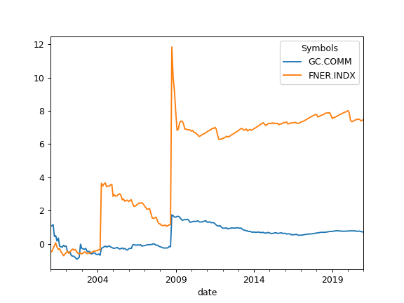
>>> al = ok.AssetList(["GC.COMM", "FNER.INDX"], first_date="2000-01", last_date="2021-01")
>>> al.names
{'GC.COMM': 'Gold',
'FNER.INDX': 'FTSE NAREIT All Equity REITs'}
>>> al.jarque_bera
            GC.COMM   FNER.INDX
statistic  4.507287  593.633047
p-value    0.105016    0.000000
Gold return time series (GC.COMM) distribution have small p-values (H0 is not rejected). Null hypothesis (H0) is rejected for FTSE NAREIT Index (FNER.INDX) as Jarque-Bera test shows very small p-value and large statistic.
- kstest(distr='norm')
Perform Kolmogorov-Smirnov test for goodness of fit the asset returns to a given distribution.
Kolmogorov-Smirnov is a test of the distribution of assets returns historical data against a given distribution. Under the null hypothesis (H0), the two distributions are identical.
- Parameters:
- distr{‘norm’, ‘lognorm’, ‘t’}, default ‘norm’
Distribution type for the rate of return of portfolio. ‘norm’ - for normal distribution. ‘lognorm’ - for lognormal distribution. ‘t’ - for Student’s T distribution.
- Returns:
- DataFrame
Returns test statistic and the p-value for the hypothesis test. Large test statistics and tiny p-value (< 0.05) indicate that null hypothesis (H0) is rejected.
Examples
>>> al = ok.AssetList(["EDV.US"], last_date="2021-01")
>>> al.kstest(distr="lognorm")
             EDV.US
p-value    0.402179
statistic  0.070246
H0 is not rejected for EDV ETF and it seems to have lognormal distribution.
- property kurtosis
Calculate expanding Fisher (normalized) kurtosis of the return time series for each asset.
Kurtosis is the fourth central moment divided by the square of the variance. It is a measure of the “tailedness” of the probability distribution of a real-valued random variable.
Kurtosis should be close to zero for normal distribution.
- Returns:
- DataFrame
Expanding kurtosis time series for each asset.
See also
skewnessCompute skewness.
skewness_rollingCompute rolling skewness.
kurtosis_rollingCalculate rolling Fisher (normalized) kurtosis.
jarque_beraPerform Jarque-Bera test for normality.
kstestPerform Kolmogorov-Smirnov test for different types of distributions.
Examples
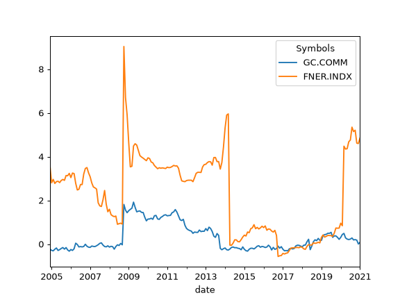
>>> import matplotlib.pyplot as plt
>>> al = ok.AssetList(["GC.COMM", "FNER.INDX"], first_date="2000-01", last_date="2021-01")
>>> al.names
{'GC.COMM': 'Gold',
'FNER.INDX': 'FTSE NAREIT All Equity REITs'}
>>> al.kurtosis.plot()
>>> plt.show()
- kurtosis_rolling(window=60)
Calculate rolling Fisher (normalized) kurtosis of the return time series for each asset.
Kurtosis is the fourth central moment divided by the square of the variance. It is a measure of the “tailedness” of the probability distribution of a real-valued random variable.
Kurtosis should be close to zero for normal distribution.
- Parameters:
- windowint, default 60
Rolling window size in months. This is the number of observations used for calculating the statistic. The window size should be at least 12 months.
- Returns:
- DataFrame
Rolling kurtosis time series for each asset.
See also
skewnessCompute skewness.
skewness_rollingCompute rolling skewness.
kurtosisCalculate expanding Fisher (normalized) kurtosis.
jarque_beraPerform Jarque-Bera test for normality.
kstestPerform Kolmogorov-Smirnov test for different types of distributions.
Examples
>>> import matplotlib.pyplot as plt
>>> al = ok.AssetList(["GC.COMM", "FNER.INDX"], first_date="2000-01", last_date="2021-01")
>>> al.names
{'GC.COMM': 'Gold',
'FNER.INDX': 'FTSE NAREIT All Equity REITs'}
>>> al.kurtosis_rolling(window=12 * 5).plot()
>>> plt.show()
- property mean_return
Calculate annualized mean return (arithmetic mean) for the rate of return time series (each asset).
Mean return calculated for the full history period. Arithmetic mean for the inflation is also shown if there is an inflation=True option in AssetList.
- Returns:
- Series
Mean return value for each asset.
Examples
>>> x = ok.AssetList(["MCFTR.INDX", "RGBITR.INDX"], ccy="RUB", inflation=True)
>>> x.mean_return
MCFTR.INDX     0.209090
RGBITR.INDX    0.100133
dtype: float64
- plot_assets(kind='mean', tickers='tickers', pct_values=False, xy_text=(0, 10), **kwargs)
Plot asset points on the risk-return chart with annotations.
Annualized values for risk and return are used. Risk is the standard deviation of monthly rate of return time series. Return can be an annualized mean return (expected return) or CAGR (compound annual growth rate).
- Parameters:
- kind{‘mean’, ‘cagr’}, default ‘mean’
Type of return: annualized mean return (expected return) or CAGR (compound annual growth rate).
- tickers{‘tickers’, ‘names’, ‘local_names’} or list of str, default ‘tickers’
Annotation type for assets.
‘tickers’: asset symbols are shown in the form ‘SPY.US’.
‘names’: asset names are shown (for example, ‘SPDR S&P 500 ETF Trust’).
‘local_names’: native-language names (e.g. ‘Сбербанк’ / ‘贵州茅台’).
list of str: custom annotations for each asset.
Note
Rendering native (‘local_names’) labels written in CJK scripts (Chinese, Japanese, Korean) requires a CJK-capable matplotlib font; with the default fonts such glyphs appear as tofu boxes.
- pct_valuesbool, default False
If True, show risk and return values in percent. If False, show values as decimals.
- xy_texttuple, default (0, 10)
The shift of the annotation text (x, y) from the point.
- **kwargs
Arbitrary keyword arguments passed to matplotlib.pyplot.scatter.
- Returns:
- Axes
Matplotlib axes object.
Examples
>>> import matplotlib.pyplot as plt
>>> al = ok.AssetList(["SPY.US", "AGG.US"], ccy="USD", inflation=False)
>>> al.plot_assets()
>>> plt.show()
Plotting with default parameters values shows expected return, ticker annotations and algebraic values for risk and return. To use CAGR instead of expected return use kind=’cagr’.
>>> al.plot_assets(
...     kind="cagr",
...     tickers=["US Stocks", "US Bonds"],  # use custom annotations for the assets
...     pct_values=True,  # risk and return values are in percents
... )
>>> plt.show()
- property price_drawdowns
Calculate price drawdowns time series for the assets.
The price drawdown is the percent decline from a previous peak in close price. Close prices are not adjusted for corporate actions (dividends and splits), hence price drawdowns may significantly differ from drawdowns (based on total return) for assets with high dividends.
- Returns:
- DataFrame
Time series of price drawdowns.
See also
drawdownsCalculate drawdowns from total return (with dividends reinvested).
Examples
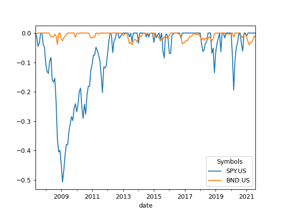
>>> import matplotlib.pyplot as plt
>>> al = ok.AssetList(["SPY.US", "BND.US"], last_date="2021-08")
>>> al.price_drawdowns.plot()
>>> plt.show()
- property real_drawdowns
Calculate real (inflation-adjusted) drawdowns time series for the assets.
The real drawdown is the percent decline from a previous peak in the inflation-adjusted wealth index. AssetList should be initiated with inflation=True for real drawdowns.
- Returns:
- DataFrame
Time series of real drawdowns.
See also
drawdownsCalculate drawdowns (not adjusted for inflation).
Examples
>>> import matplotlib.pyplot as plt
>>> al = ok.AssetList(["SPY.US", "BND.US"], inflation=True, last_date="2021-08")
>>> al.real_drawdowns.plot()
>>> plt.show()

- property real_mean_return
Calculate annualized real mean return (arithmetic mean) for the rate of return time series (each assets).
Real rate of return is adjusted for inflation. Real return is defined if there is an inflation=True option in AssetList.
- Returns:
- Series
Mean real return value for each asset.
Examples
>>> x = ok.AssetList(["MCFTR.INDX", "RGBITR.INDX"], ccy="RUB", inflation=True)
>>> x.real_mean_return
MCFTR.INDX     0.118116
RGBITR.INDX    0.017357
dtype: float64
- property recovery_periods
Calculate the longest recovery periods for the assets.
The recovery period (drawdown duration) is the number of months to reach the value of the last maximum.
- Returns:
- Series
Max recovery period for each asset (in months).
See also
drawdownsCalculate drawdowns time series.
Notes
If the last asset maximum value is not recovered NaN is returned. The largest recovery period does not necessary correspond to the max drawdown.
Examples
>>> x = ok.AssetList(["SPY.US", "AGG.US"])
>>> x.recovery_periods
SPY.US    52
AGG.US    15
dtype: int32
- property risk_annual
Calculate annualized risk expanding time series for each asset.
Risk is a standard deviation of the rate of return.
Annualized risk time series is calculated for the rate of return from ‘first_date’ to ‘last_date’ (expanding).
- Returns:
- DataFrame
Annualized risk (standard deviation) expanding time series for each asset.
See also
risk_monthlyCalculate montly risk expanding time series for each asset.
get_rolling_risk_annualCalculate annualized risk rolling time series.
semideviation_monthlyCalculate semideviation monthly values.
semideviation_annualCalculate semideviation annualized values.
get_var_historicCalculate historic Value at Risk (VaR).
get_cvar_historicCalculate historic Conditional Value at Risk (CVaR).
drawdownsCalculate assets drawdowns.
Notes
CFA recomendations are used to annualize risk values [1].
[1]What’s Wrong with Multiplying by the Square Root of Twelve. Paul D. Kaplan, CFA Institute Journal Review, 2013
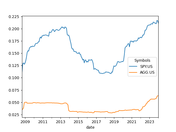
Examples
>>> al = ok.AssetList(["GC.COMM", "SHV.US"], ccy="USD", last_date="2021-01")
>>> al.risk_annual
Symbols   GC.COMM    SHV.US
date
2007-03  0.097820  0.000511
2007-04  0.084806  0.000552
2007-05  0.099466  0.001633
2007-06  0.089265  0.001472
2007-07  0.095290  0.001442
...           ...       ...
2020-09  0.193815  0.004824
2020-10  0.193087  0.004813
2020-11  0.192583  0.004807
2020-12  0.193513  0.004796
2021-01  0.192754  0.004788
[167 rows x 2 columns]
- property risk_monthly
Calculate monthly risk expanding time series for each asset.
Monthly risk of the asset is a standard deviation of the rate of return time series. Standard deviation (sigma σ) is normalized by N-1.
Monthly risk is calculated for the rate of retirun time series for the sample from ‘first_date’ to ‘last_date’.
- Returns:
- DataFrame
Monthly risk (standard deviation) expanding time series for each asset in form of Series.
See also
risk_annualCalculate annualized risks expanding time series.
semideviation_monthlyCalculate semideviation monthly values.
semideviation_annualCalculate semideviation annualized values.
get_var_historicCalculate historic Value at Risk (VaR).
get_cvar_historicCalculate historic Conditional Value at Risk (CVaR).
drawdownsCalculate drawdowns.
Examples
>>> al = ok.AssetList(["GC.COMM", "SHV.US"], ccy="USD", last_date="2021-01")
>>> al.risk_monthly
Symbols   GC.COMM    SHV.US
date
2007-03  0.025668  0.000141
2007-04  0.020872  0.000153
2007-05  0.027513  0.000451
2007-06  0.025988  0.000406
           ...       ...
2020-09  0.051006  0.001380
2020-10  0.050861  0.001377
- property semideviation_annual
Return semideviation annualized values for each asset.
Semi-deviation (Downside risk) is the risk of the return being below the expected return.
Semi-deviation is calculated for rate of retirun time series for the sample from ‘first_date’ to ‘last_date’.
- Returns:
- Series
Annualized semideviation values for each asset in form of Series.
See also
risk_monthlyCalculate montly risk for each asset.
risk_annualCalculate annualized risks.
semideviation_monthlyCalculate semideviation monthly values.
get_var_historicCalculate historic Value at Risk (VaR).
get_cvar_historicCalculate historic Conditional Value at Risk (CVaR).
drawdownsCalculate drawdowns.
Examples
>>> al = ok.AssetList(["GC.COMM", "SHV.US"], ccy="USD", last_date="2021-01")
>>> al.semideviation_annual
GC.COMM    0.112411
SHV.US     0.001052
dtype: float64
- property semideviation_monthly
Calculate semi-deviation monthly values for each asset.
Semi-deviation (Downside risk) is the risk of the return being below the expected return.
Semi-deviation is calculated for rate of retirun time series for the sample from ‘first_date’ to ‘last_date’.
- Returns:
- Series
Monthly semideviation values for each asset in form of Series.
See also
risk_monthlyCalculate montly risk for each asset.
risk_annualCalculate annualized risks.
semideviation_annualCalculate semideviation annualized values.
get_var_historicCalculate historic Value at Risk (VaR).
get_cvar_historicCalculate historic Conditional Value at Risk (CVaR).
drawdownsCalculate drawdowns.
Examples
>>> al = ok.AssetList(["GC.COMM", "SHV.US"], ccy="USD", last_date="2021-01")
>>> al.semideviation_monthly
GC.COMM    0.032450
SHV.US     0.000304
dtype: float64
- property skewness
Compute expanding skewness of the return time series for each asset returns.
Skewness is a measure of the asymmetry of the probability distribution of a real-valued random variable about its mean. The skewness value can be positive, zero, negative, or undefined.
For normally distributed returns, the skewness should be about zero. A skewness value greater than zero means that there is more weight in the right tail of the distribution.
- Returns:
- Dataframe
Expanding skewness time series for each asset.
See also
skewness_rollingCompute rolling skewness.
kurtosisCalculate expanding Fisher (normalized) kurtosis.
kurtosis_rollingCalculate rolling Fisher (normalized) kurtosis.
jarque_beraPerform Jarque-Bera test for normality.
kstestPerform Kolmogorov-Smirnov test for different types of distributions.
Examples
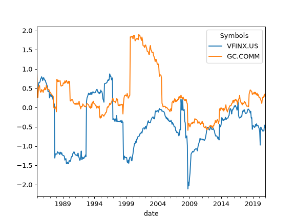
>>> import matplotlib.pyplot as plt
>>> al = ok.AssetList(["VFINX.US", "GC.COMM"], last_date="2021-01")
>>> al.names
{'VFINX.US': 'VANGUARD 500 INDEX FUND INVESTOR SHARES',
'GC.COMM': 'Gold'}
>>> al.skewness.plot()
>>> plt.show()
- skewness_rolling(window=60)
Compute rolling skewness of the return time series for each asset.
Skewness is a measure of the asymmetry of the probability distribution of a real-valued random variable about its mean. The skewness value can be positive, zero, negative, or undefined.
For normally distributed returns, the skewness should be about zero. A skewness value greater than zero means that there is more weight in the right tail of the distribution.
- Parameters:
- windowint, default 60
Rolling window size in months. This is the number of observations used for calculating the statistic. The window size should be at least 12 months.
- Returns:
- DataFrame
Rolling skewness time series for each asset.
See also
skewnessCompute skewness.
kurtosisCalculate expanding Fisher (normalized) kurtosis.
kurtosis_rollingCalculate rolling Fisher (normalized) kurtosis.
jarque_beraPerform Jarque-Bera test for normality.
kstestPerform Kolmogorov-Smirnov test for different types of distributions.
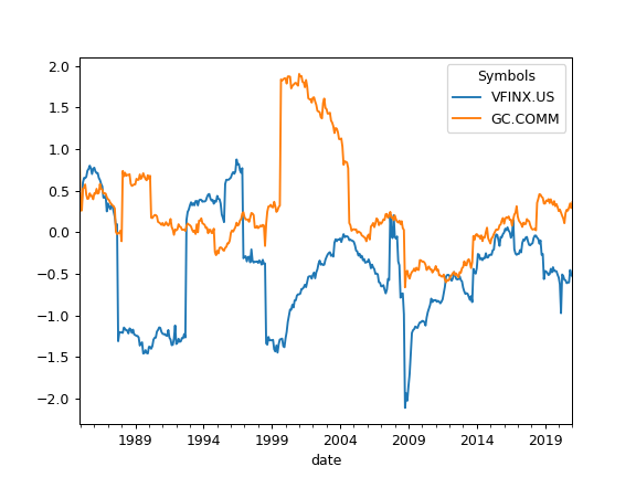
Examples
>>> import matplotlib.pyplot as plt
>>> al = ok.AssetList(["VFINX.US", "GC.COMM"], last_date="2021-01")
>>> al.names
{'VFINX.US': 'VANGUARD 500 INDEX FUND INVESTOR SHARES',
'GC.COMM': 'Gold'}
>>> al.skewness_rolling(window=12 * 5).plot()
>>> plt.show()
- property symbols
Return a list of used financial symbols.
Symbols are similar to tickers but have a namespace information:
SPY.US is a symbol
SPY is a ticker
- Returns:
- list of str
List of used symbols.
- property tickers
Return a list of used tickers (symbols without a namespace).
Tickers are similar to symbols but do not have namespace information:
SPY is a ticker
SPY.US is a symbol
- Returns:
- list of str
List of used tickers.
- tracking_difference(rolling_window=None)
Return tracking difference for the rate of return of assets.
Tracking difference is calculated by measuring the accumulated difference between the returns of a benchmark and those of the ETF replicating it (could be mutual funds, or other types of assets). Tracking difference is measured in percents.
Benchmark should be in the first position of the symbols list in AssetList parameters.
- Parameters:
- rolling_windowint or None, default None
Size of the moving window in months. If None calculate expanding tracking difference.
- Returns:
- DataFrame
Tracking diffirence time series for each asset.
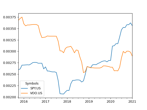
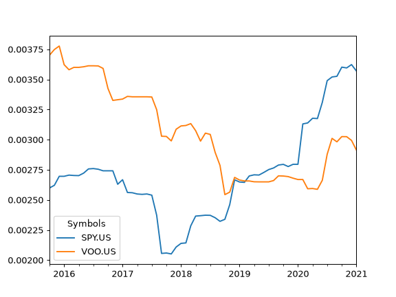
Examples
>>> import matplotlib.pyplot as plt
>>> x = ok.AssetList(["SP500TR.INDX", "SPY.US", "VOO.US"], last_date="2021-01")
>>> x.tracking_difference().plot()
>>> plt.show()
To calculate rolling Tracking difference set rolling_window to a number of months (moving window size):
>>> x.tracking_difference(rolling_window=24).plot()
>>> plt.show()
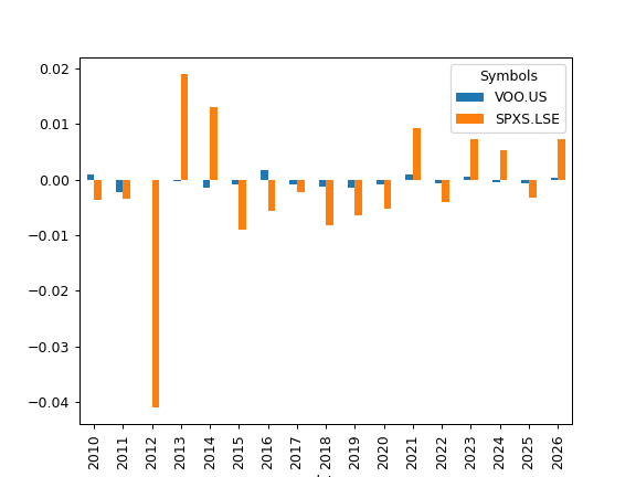
- property tracking_difference_annual
Calculate tracking difference for each calendar year.
Tracking difference is calculated by measuring the accumulated difference between the returns of a benchmark and ETFs replicating it (could be mutual funds, or other types of assets). Tracking difference is measured in percents.
Benchmark should be in the first position of the symbols list in AssetList parameters.
- Returns:
- DataFrame
Time series with tracking difference for each calendar year period.
Examples
>>> import matplotlib.pyplot as plt
>>> al = ok.AssetList(["SP500TR.INDX", "VOO.US", "SPXS.LSE"], inflation=False)
>>> al.tracking_difference_annual.plot(kind="bar")
- tracking_difference_annualized(rolling_window=None)
Calculate annualized tracking difference time series for the rate of return of assets.
Tracking difference is calculated by measuring the accumulated difference between the returns of a benchmark and ETFs replicating it (could be mutual funds, or other types of assets). Tracking difference is measured in percents.
Benchmark should be in the first position of the symbols list in AssetList parameters.
Annual values are available for history periods of more than 12 months. Returns for less than 12 months can’t be annualized According to the CFA Institute’s Global Investment Performance Standards (GIPS).
- Parameters:
- rolling_windowint or None, default None
Size of the moving window in months. Must be at least 12 months. If None calculate expanding annualized tracking difference.
- Returns:
- DataFrame
Annualized tracking diffirence time series for each asset.
Examples
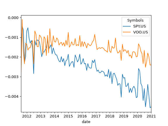
>>> import matplotlib.pyplot as plt
>>> x = ok.AssetList(["SP500TR.INDX", "SPY.US", "VOO.US"], last_date="2021-01")
>>> x.tracking_difference_annualized().plot()
To calculate rolling annualized tracking difference set rolling_window to a number of months (moving window size):
>>> x.tracking_difference_annualized(rolling_window=12 * 5).plot()
>>> plt.show()
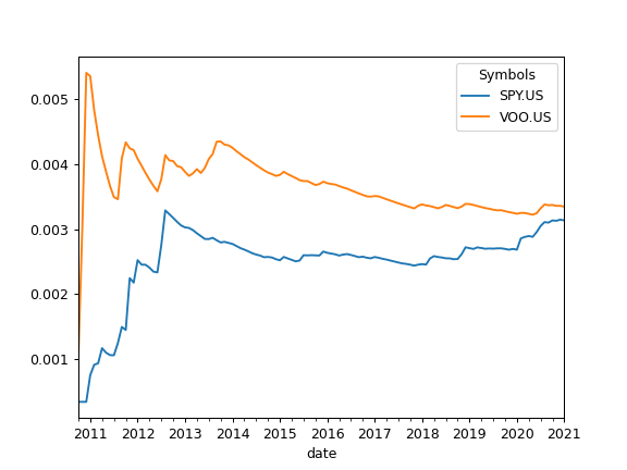
- tracking_error(rolling_window=None, method='rms')
Calculate tracking error time series for the rate of return of assets.
Tracking error is an ex-post measure of how closely the assets follow the benchmark. It is computed from the realized monthly return differences between each asset and the benchmark, and is annualized (multiplied by sqrt(12)). Tracking error values are decimal fractions: 0.05 corresponds to 5% annualized.
Benchmark should be in the first position of the symbols list in AssetList parameters.
Two formulas are available (method parameter):
“rms” (default): root-mean-square of the return differences. The differences are not centered around their mean, hence the systematic lag between an asset and the benchmark (tracking difference) is included in the result.
“std”: sample standard deviation of the return differences with Bessel’s correction — the classic tracking error definition (Hwang & Satchell, “Tracking Error: Ex-Ante versus Ex-Post Measures”, 2001, eq. 2) measuring the pure volatility of deviations from the benchmark. The first point of the expanding time series is dropped (a single observation has no standard deviation).
- Parameters:
- rolling_windowint or None, default None
Size of the moving window in months. Must be at least 12 months. If None calculate expanding tracking error.
- method{“rms”, “std”}, default “rms”
Tracking error formula: “rms” for the uncentered root-mean-square of return differences, “std” for the centered sample standard deviation.
- Returns:
- DataFrame
rolling or expanding tracking error time series for each asset.
Examples
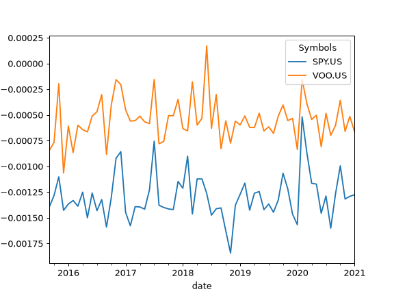
>>> import matplotlib.pyplot as plt
>>> x = ok.AssetList(["SP500TR.INDX", "SPY.US", "VOO.US"], last_date="2021-01")
>>> x.tracking_error().plot()
>>> plt.show()

To calculate rolling tracking error set rolling_window to a number of months (moving window size):
>>> x.tracking_error(rolling_window=12 * 5, method="std").plot()
>>> plt.show()
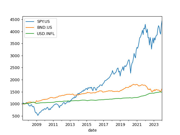
- property wealth_indexes
Calculate wealth index time series for the assets and accumulated inflation.
Wealth index (Cumulative Wealth Index) is a time series that presents the value of each asset over historical time period. Accumulated inflation time series is added if inflation=True in the AssetList.
Wealth index is obtained from the accumulated return multiplied by the initial investments. That is: 1000 * (Acc_Return + 1) Initial investments are taken as 1000 units of the AssetList base currency.
- Returns:
- DataFrame
Time series of wealth index values for each asset and accumulated inflation.
Examples
>>> import matplotlib.pyplot as plt
>>> x = ok.AssetList(["SPY.US", "BND.US"])
>>> x.wealth_indexes.plot()
>>> plt.show()
- property target_risk_range
Calculate range of annualized risk values (from min risk to max risk).
The number of values in the range is defined by ‘n_points’. The risk is defined as standard deviation of monthly rate or returns time series.
- Returns:
- numpy.ndarray
Annualized risk values (from min risk to max risk)
Examples
>>> frontier = ok.EfficientFrontier(["SPY.US", "AGG.US"])
>>> frontier.target_risk_range
array([0.03695845, 0.04334491, 0.04973137, 0.05611783, 0.06250429,
       0.06889075, 0.07527721, 0.08166367, 0.08805012, 0.09443658,
       0.10082304, 0.1072095 , 0.11359596, 0.11998242, 0.12636888,
       0.13275534, 0.1391418 , 0.14552826, 0.15191472, 0.15830117])
- property ef_points
Generate multi-period Efficient Frontier.
Each point on the Efficient Frontier is a rebalanced portfolio with optimized annual risk for a given CAGR. In case of non-convexity along the risk axis, the second part of the chart is generated, where the maximum risk value is found for each point.
- Returns:
- DataFrame
Table of weights and risk/return values for the Efficient Frontier. The columns:
assets weights
CAGR
Risk (standard deviation)
All the values are annualized.
Examples
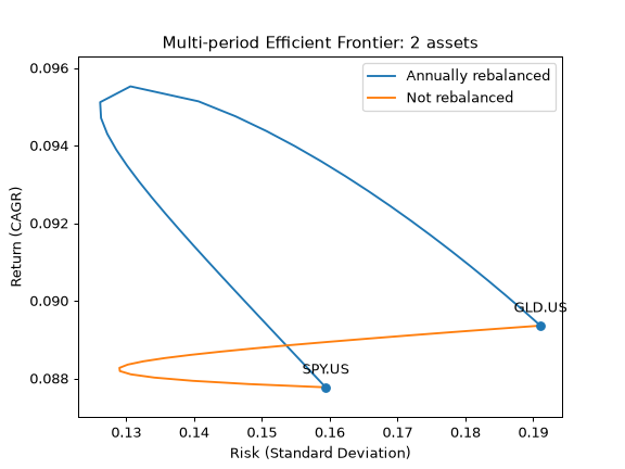
>>> ls = ["SPY.US", "GLD.US"]
>>> curr = "USD"
>>> y = ok.EfficientFrontier(
...     assets=ls,
...     first_date="2004-12",
...     last_date="2020-10",
...     ccy=curr,
...     rebalancing_strategy=ok.Rebalance(period="year"),
...     ticker_names=True,  # Use tickers in DataFrame column names.
...     n_points=20,  # Number of points in the Efficient Frontier.
... )
>>> df_reb_year = y.ef_points
>>> df_reb_year[["Risk", "CAGR", "SPY.US", "GLD.US"]].head(5)
       Risk      CAGR    SPY.US    GLD.US
0  0.159403  0.087770  1.000000  0.000000
1  0.157208  0.088178  0.985742  0.014258
2  0.155011  0.088586  0.971065  0.028935
3  0.152814  0.088994  0.955931  0.044069
4  0.150619  0.089402  0.940300  0.059700
To compare the Efficient Frontiers of annually rebalanced portfolios with not rebalanced portfolios it’s possible to draw 2 charts: rebalancing_strategy=ok.Rebalance(period=’year’) and ok.Rebalance(period=’none’).
>>> import matplotlib.pyplot as plt
>>> y.rebalancing_strategy = ok.Rebalance(period="none")
>>> df_not_reb = y.ef_points
>>> fig = plt.figure()
>>> # Plot the assets points using CAGR to match the Efficient Frontier Y-axis.
>>> ax = y.plot_assets(kind="cagr")
>>> # Plot the Efficient Frontier for annually rebalanced portfolios
>>> ax.plot(df_reb_year["Risk"], df_reb_year["CAGR"], label="Annually rebalanced")
>>> # Plot the Efficient Frontier for not rebalanced portfolios
>>> ax.plot(df_not_reb["Risk"], df_not_reb["CAGR"], label="Not rebalanced")
>>> # Set axis labels and the title
>>> ax.set_title("Multi-period Efficient Frontier: 2 assets")
>>> ax.set_xlabel("Risk (Standard Deviation)")
>>> ax.set_ylabel("Return (CAGR)")
>>> ax.legend()
>>> plt.show()
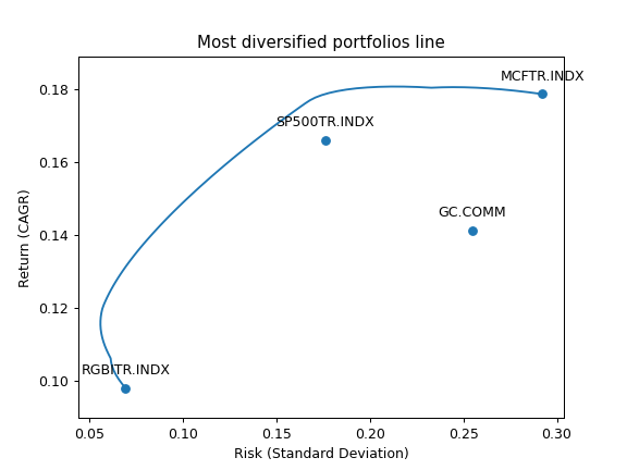
- property mdp_points
Generate Most diversified portfolios frontier for rebalanced portfolios.
Each point on the Most diversified portfolios frontier is a rebalanced portfolio with optimized Diversification ratio for a given CAGR.
The points are obtained through the constrained optimization process (optimization with bounds). Bounds are defined with ‘bounds’ property.
- Returns:
- DataFrame
Table of weights and risk/return values for the Most Diversified Portfolios Frontier. The columns:
assets weights
CAGR (geometric mean)
Risk (standard deviation)
Diversification ratio
All the values are annualized.
Examples
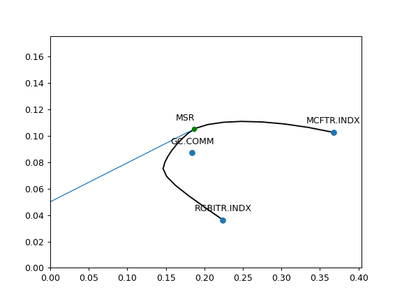
>>> ls4 = ["SP500TR.INDX", "MCFTR.INDX", "RGBITR.INDX", "GC.COMM"]
>>> y = ok.EfficientFrontier(assets=ls4, ccy="RUB", last_date="2021-12", n_points=20)
>>> y.mdp_points  # print mdp weights, risk, CAGR and Diversification ratio
        Risk      CAGR  Diversification ratio  ...    MCFTR.INDX   RGBITR.INDX  SP500TR.INDX
0   0.066040  0.092220               1.234567  ...  2.081668e-16  1.000000e+00  0.000000e+00
1   0.064299  0.093451               1.245678  ...  0.000000e+00  9.844942e-01  5.828671e-16
...
To plot the Most diversification portfolios line use the DataFrame with the points data. Additionally ‘Plot.plot_assets()’ can be used to show the assets in the chart.
>>> import matplotlib.pyplot as plt
>>> fig = plt.figure()
>>> # Plot the assets points
>>> y.plot_assets(kind="cagr")  # kind should be set to "cagr" as we take "CAGR" column from the mdp_points.
>>> ax = plt.gca()
>>> # Plot the Most diversified portfolios line
>>> df = y.mdp_points
>>> ax.plot(df["Risk"], df["CAGR"])  # we chose to plot CAGR which is geometric mean of return series
>>> # Set the axis labels and the title
>>> ax.set_title("Most diversified portfolios line")
>>> ax.set_xlabel("Risk (Standard Deviation)")
>>> ax.set_ylabel("Return (CAGR)")
>>> plt.show()
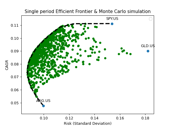
- get_monte_carlo(n=100)
Generate random rebalanced portfolios with Monte Carlo simulation.
Risk (annualized standard deviation) and return (CAGR) are calculated for random weights within bounds.
- Parameters:
- nint, default 100
Number of random portfolios to generate with Monte Carlo simulation.
- Returns:
- DataFrame
Table with Return (CAGR) and Risk values for random portfolios (portfolios with random asset weights).
Examples
>>> ls_m = ["SPY.US", "GLD.US", "PGJ.US", "RGBITR.INDX", "MCFTR.INDX"]
>>> curr_rub = "RUB"
>>> x = ok.EfficientFrontier(
...     assets=ls_m,
...     first_date="2005-01",
...     last_date="2020-11",
...     ccy=curr_rub,
...     rebalancing_strategy=ok.Rebalance(period="year"),  # set rebalancing period to one year
...     n_points=20,
...     verbose=False,
... )
>>> monte_carlo = x.get_monte_carlo(n=1000)  # it can take some time ...
>>> monte_carlo.head(5)
       CAGR      Risk
0  0.182937  0.178518
1  0.184915  0.172965
2  0.154892  0.141681
3  0.185500  0.168739
4  0.176748  0.192657
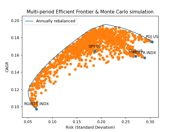
Monte Carlo simulation results can be plotted together with the optimized portfolios on the Efficient Frontier.
>>> import matplotlib.pyplot as plt
>>> df_reb_year = x.ef_points  # optimize portfolios for EF. Calculations will take some time ...
>>> fig = plt.figure()
>>> # Plot the assets points (optional).
>>> x.plot_assets(kind="cagr")
>>> ax = plt.gca()
>>> # Plot random portfolios (Monte Carlo simulation)
>>> ax.scatter(monte_carlo.Risk, monte_carlo.CAGR)
>>> # Plot the Efficient Frontier
>>> ax.plot(df_reb_year.Risk, df_reb_year.CAGR, label="Annually rebalanced")
>>> # Set the axis labels and Title
>>> ax.set_title("Multi-period Efficient Frontier & Monte Carlo simulation")
>>> ax.set_xlabel("Risk (Standard Deviation)")
>>> ax.set_ylabel("CAGR")
>>> ax.legend()
>>> plt.show()
- get_grid_portfolios(step=0.1, max_points=100000)
Generate rebalanced portfolios for all weight combinations on a grid.
Weights are enumerated with a fixed step that must divide 1.0 evenly (e.g. 0.05, 0.10, 0.20, 0.25, 0.50). Per-asset
boundsare respected.- Parameters:
- stepfloat, default 0.10
Weight increment (e.g. 0.10 for 10 %).
- max_pointsint, default 100_000
Guardrail on the number of grid portfolios. The point count grows combinatorially with the number of assets and
1 / step; an oversized request raisesValueErrorbefore enumeration instead of hanging. Raise it to allow larger grids at the cost of runtime.
- Returns:
- DataFrame
Table with Risk (annualized std) and CAGR for every grid portfolio.
Examples
>>> ls_m = ["SPY.US", "GLD.US"]
>>> x = ok.EfficientFrontier(
...     assets=ls_m,
...     first_date="2005-01",
...     last_date="2020-11",
...     ccy="USD",
...     rebalancing_strategy=ok.Rebalance(period="year"),
... )
>>> grid = x.get_grid_portfolios(step=0.25)
>>> grid.head()
       CAGR      Risk
0  ...       ...
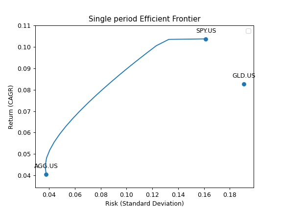
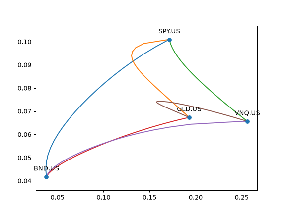
- plot_pair_ef(tickers='tickers', figsize=None)
Plot Efficient Frontier for every pair of assets.
Efficient Frontier is a set of portfolios which satisfy the condition that no other portfolio exists with a higher expected return but with the same risk (standard deviation of return).
- Parameters:
- tickers{‘tickers’, ‘names’, ‘local_names’} or list[str], default ‘tickers’
Annotation type for assets. ‘tickers’ - assets symbols are shown in form of ‘SPY.US’ ‘names’ - assets names are used like - ‘SPDR S&P 500 ETF Trust’ ‘local_names’ - native-language names (e.g. ‘Сбербанк’ / ‘贵州茅台’) To show custom annotations for each asset pass the list of names.
- figsizetuple[float, float], default None
Figure size (width, height) in inches. If None, matplotlib default is used.
- Returns:
- Axes
Matplotlib axes with the plot.
Notes
At least 3 assets are required.
Examples
>>> import matplotlib.pyplot as plt
>>> ls4 = ["SPY.US", "BND.US", "GLD.US", "VNQ.US"]
>>> curr = "USD"
>>> last_date = "2021-07"
>>> ef = ok.EfficientFrontier(ls4, ccy=curr, last_date=last_date)
>>> ef.plot_pair_ef()
>>> plt.show()
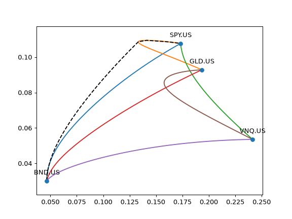
It can be useful to plot the full Efficient Frontier (EF) with optimized 4 asset portfolios together with the EFs for each pair of assets.
>>> ef4 = ok.EfficientFrontier(assets=ls4, ccy=curr, n_points=100)
>>> df4 = ef4.ef_points
>>> fig = plt.figure()
>>> # Plot Efficient Frontier for every pair of assets. Optimized portfolios will have 2 assets.
>>> ef4.plot_pair_ef()  # CAGR is used for optimized portfolios.
>>> ax = plt.gca()
>>> # Plot the full Efficient Frontier for 4 asset portfolios.
>>> ax.plot(df4["Risk"], df4["CAGR"], color="black", linestyle="--")
>>> plt.show()

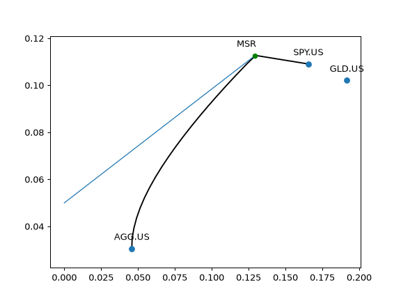
- plot_cml(rf_return=0, figsize=None)
Plot Capital Market Line (CML).
The Capital Market Line (CML) is the tangent line drawn from the point of the risk-free asset (volatility is zero) to the point of tangency portfolio or Maximum Sharpe Ratio (MSR) point.
The slope of the CML is the Sharpe ratio of the tangency portfolio.
- Parameters:
- rf_returnfloat, default 0
Risk-free rate of return.
- figsizetuple[float, float], default None
Figure size (width, height) in inches. If None, matplotlib default is used.
- Returns:
- Axes
Matplotlib axes with the plot.
Examples
>>> import matplotlib.pyplot as plt
>>> three_assets = ["SPY.US", "AGG.US", "GLD.US"]
>>> ef = ok.EfficientFrontier(assets=three_assets, ccy="USD", full_frontier=True)
>>> ef.plot_cml(rf_return=0.05)  # Risk-Free return is 5%
>>> plt.show()
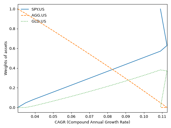
- plot_transition_map(x_axe='risk', figsize=None)
Plot Transition Map for optimized portfolios on the Efficient Frontier.
Transition Map shows the relation between asset weights and optimized portfolio properties:
CAGR (Compound annual growth rate)
Risk (annualized standard deviation of return)
- Parameters:
- x_axe{‘risk’, ‘cagr’}, default ‘risk’
Show the relation between weights and CAGR (if ‘cagr’) or between weights and Risk (if ‘risk’). CAGR or Risk are displayed on the x-axis.
- figsizetuple[float, float], default None
Figure size (width, height) in inches. If None, matplotlib default is used.
- Returns:
- Axes
Matplotlib axes with the plot.
Examples
>>> import matplotlib.pyplot as plt
>>> x = ok.EfficientFrontier(["SPY.US", "AGG.US", "GLD.US"], ccy="USD", inflation=False)
>>> x.plot_transition_map()
>>> plt.show()
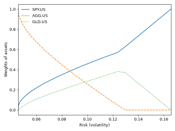
Transition Map with default settings shows the relation between risk (standard deviation) and asset weights for optimized portfolios. The same relation for CAGR can be shown by setting x_axe=’cagr’.
>>> x.plot_transition_map(x_axe="cagr")
>>> plt.show()