okama.PortfolioDCF

class PortfolioDCF(parent)

Bases: object

Class to access discounted cash flow (DCF) methods of Portfolio. All methods can be used in Portfolio instances trough construction: ` pf = Portfolio() pf.dcf.weatlh_index pf.dсf.cashflow_pv `

Methods & Attributes

`cashflow_pv`	Calculate the discounted value (PV) of the cash flow amount at the historical first date.
`initial_amount_pv`	Calculate the discounted value (PV) of the initial investments at the historical first date.
`monte_carlo_survival_period`([distr, years, n])	Generate a survival period distribution for a portfolio with cash flows by Monte Carlo simulation.
`plot_forecast_monte_carlo`([distr, years, ...])	Plot Monte Carlo simulation for portfolio future wealth indexes optionally together with historical wealth index.
`survival_date`	Get the date when the portfolio balance become negative considering withdrawals on the historical data.
`survival_period`	Calculate the period when the portfolio has positive balance considering withdrawals on the historical data.
`wealth_index`	Calculate wealth index time series for the portfolio with contributions and withdrawals.

property wealth_index

Calculate wealth index time series for the portfolio with contributions and withdrawals.

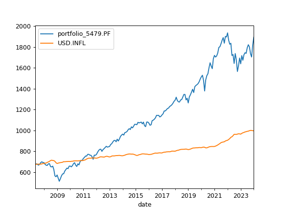
Wealth index (Cumulative Wealth Index) is a time series that presents the value of portfolio over historical time period considering cash flows.

Accumulated inflation time series is added if inflation=True in the Portfolio.

If there is no cashflows Wealth index is obtained from the accumulated return multiplicated by the initial investments. That is: initial_amount_pv * (Acc_Return + 1)

initial_amount_pv is the discounted value of the initial investments (initial_amount).

Values of the wealth index correspond to the beginning of the month.

Returns:

Time series of wealth index values for portfolio and accumulated inflation.

Examples

>>> import matplotlib.pyplot as plt
>>> x = ok.Portfolio(['SPY.US', 'BND.US'])
>>> x.dcf.wealth_index.plot()
>>> plt.show()

property survival_period

Calculate the period when the portfolio has positive balance considering withdrawals on the historical data.

The portfolio survival period (longevity period) depends on the investment strategy: asset allocation, rebalancing, withdrawals rate etc.

The withdrawals are defined by the cashflow parameter of the portfolio.

Returns:

float: The portfolio survival period (longevity period) in years.

Examples

>>> pf = ok.Portfolio(
...    ['SPY.US', 'AGG.US'],
...    ccy='USD',
...    first_date='2010-01',
...    initial_amount=100_000,
...    cashflow=-1_000
...)
>>> pf.dcf.survival_period
11.6

property survival_date

Get the date when the portfolio balance become negative considering withdrawals on the historical data.

The portfolio survival date (longevity date) depends on the investment strategy: asset allocation, rebalancing, withdrawals rate etc.

The withdrawals are defined by the cashflow parameter of the portfolio.

Returns:

pd.Timestamp: The portfolio survival date (longevity period) in years.

Examples

>>> pf = ok.Portfolio(
...    ['SPY.US', 'AGG.US'],
...    ccy='USD',
...    first_date='2010-01',
...    initial_amount=100_000,
...    cashflow=-1_000
...)
>>> pf.dcf.survival_date
Timestamp('2021-08-01 00:00:00')

property cashflow_pv

Calculate the discounted value (PV) of the cash flow amount at the historical first date.

The future value (FV) is defined by cashflow parameter. The discount rate is the average annual inflation.

Returns:

float: The discounted value (PV) of the cash flow amount at the historical first date.

Examples

>>> pf = ok.Portfolio(['SPY.US', 'AGG.US'], ccy='USD', initial_amount=100_000, cashflow=-5_000)
>>> pf.dcf.cashflow_pv
-3004

property initial_amount_pv

Calculate the discounted value (PV) of the initial investments at the historical first date.

The future value (FV) is defined by initial_amount parameter. The discount rate is the average annual inflation.

Returns:

float: The discounted value (PV) of the initial investments at the historical first date.

Examples

>>> pf = ok.Portfolio(['EQMX.MOEX', 'SBGB.MOEX'], ccy='RUB', initial_amount=100_000)
>>> pf.dcf.initial_amount_pv
73650

plot_forecast_monte_carlo(distr='norm', years=1, backtest=True, n=20, figsize=None)

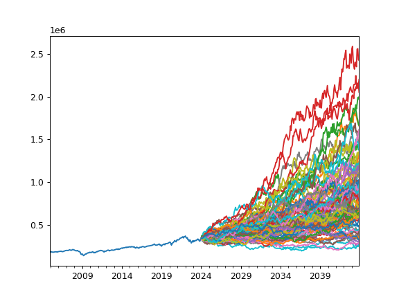
Plot Monte Carlo simulation for portfolio future wealth indexes optionally together with historical wealth index.

Wealth index (Cumulative Wealth Index) is a time series that presents the value of portfolio over time period considering cash flows (portfolio withdrawals/contributions).

Random wealth indexes are generated according to a given distribution.

Parameters:

distr{‘norm’, ‘lognorm’}, default ‘norm’: Distribution type for the rate of return of portfolio. ‘norm’ - for normal distribution. ‘lognorm’ - for lognormal distribution.
yearsint, default 1: Investment period length for new wealth indexes
backtestbool, default ‘True’: Include historical wealth index if ‘True’.
nint, default 20: Number of random wealth indexes to generate with Monte Carlo simulation.
figsize(float, float), optional: Width, height in inches. If None default matplotlib figsize value is used.

Returns:

None

Examples

>>> import matplotlib.pyplot as plt
>>> pf = ok.Portfolio(assets=['SPY.US', 'AGG.US', 'GLD.US'],
...                   weights=[.60, .35, .05],
...                   rebalancing_period='year',
...                   initial_amount=300_000,
...                   cashflow=-1_000)
>>> pf.dcf.plot_forecast_monte_carlo(years=20, backtest=True, distr='lognorm', n=100)
>>> plt.show()

monte_carlo_survival_period(distr='norm', years=1, n=20)

Generate a survival period distribution for a portfolio with cash flows by Monte Carlo simulation.

It’s possible to analyze the distribution finding “min”, “max” and percentiles to see for how long will last the investment strategy - possible longevity period.

Parameters:

distr{‘norm’, ‘lognorm’}, default ‘norm’: Distribution type for the rate of return of portfolio.
yearsint, default 1: Forecast period for portfolio wealth index time series.
nint, default 100: Number of random wealth indexes to generate with Monte Carlo simulation.

Returns:

Series: Survival period distribution for a portfolio with cash flows.

Examples

>>> pf = ok.Portfolio(
    ['SPY.US', 'AGG.US', 'GLD.US'],
    weights=[.60, .35, .05],
    rebalancing_period='year',
    initial_amount=300_000,
    cashflow=-10_000
)
>>> s = pf.dcf.monte_carlo_survival_period(
    distr="norm",
    years=10,
    n=100,
)
>>> s.min()
2.2
>>> s.max()
3.6
>> s.mean()
2.737
>> s.quantile(50 / 100)
2.7