Portfolio
- class Portfolio(assets=None, *, first_date=None, last_date=None, ccy='USD', inflation=True, weights=None, rebalancing_strategy=period month abs_deviation NaN rel_deviation NaN dtype: str, symbol=None)
Bases:
ListMakerInvestment portfolio.
An investment portfolio is a type of financial asset (same as stocks, ETFs, mutual funds, currencies, etc.). The arguments are similar to AssetList, but Portfolio additionally has:
weights
rebalancing_strategy
symbol
Portfolio is defined by the investment strategy, which includes:
asset allocation (financial assets and their proportions in the portfolio)
the rebalancing strategy (rebalancing_strategy parameter)
Rebalancing is the action of bringing the portfolio that has deviated away from the original target asset allocation back into line. After rebalancing, the portfolio assets have the original weights.
- Parameters:
- assetslist, default None
List of assets. Could include tickers or asset-like objects (Asset, Portfolio). If None, a single-asset list with a default ticker is used.
- first_datestr, default None
First date of monthly return time series. If None, the first date is calculated automatically as the oldest available date for the listed assets.
- last_datestr, default None
Last date of monthly return time series. If None, the last date is calculated automatically as the newest available date for the listed assets.
- ccystr, default ‘USD’
Base currency for the list of assets. All risk metrics and returns are adjusted to the base currency.
- inflationbool, default True
Defines whether to take inflation data into account in the calculations. Including inflation could limit available data (first_date, last_date) as the inflation data is usually published with a one-month delay. With inflation=False, some properties like real return are not available.
- weightslist of float, default None
List of asset weights. The weight of an asset is the percent of an investment portfolio that corresponds to the asset. If None, an equally weighted portfolio is created (all weights are equal).
- rebalancing_strategyRebalance, default Rebalance(period=”month”)
Rebalancing strategy for an investment portfolio. The strategy is defined by:
period (rebalancing frequency): predetermined time intervals when the investor rebalances the portfolio. If “none”, asset weights are not rebalanced.
abs_deviation: the absolute deviation allowed for the asset weights in the portfolio.
rel_deviation: the relative deviation allowed for the asset weights in the portfolio.
- symbolstr, default None
Text symbol of portfolio. It is similar to tickers but have a namespace information. Portfolio symbol must end with .PF (all_weather_portfolio.PF). If None, a random symbol is generated (portfolio_7802.PF).
Methods & Attributes
annual_return_ts([return_type])Calculate annual rate of return time series for portfolio.
Show assets monthly close time series adjusted to the base currency.
Calculate last twelve months (LTM) dividend yield time series (monthly) for each asset.
Rate of return monthly time series for all assets.
Portfolio size monthly time series.
Return the base currency.
describe([years])Generate descriptive statistics for the portfolio.
Calculate Diversification Ratio for the portfolio.
Calculate last twelve months (LTM) dividend yield time series for the portfolio.
Calculate last twelve months (LTM) dividend yield annual time series.
Calculate portfolio dividends monthly time series.
Return calendar year dividends sum time series for each asset.
Calculate drawdowns time series for the portfolio.
get_cagr([period, real])Calculate the expanding portfolio Compound Annual Growth Rate (CAGR) time series.
get_cumulative_return([period, real])Calculate the expanding cumulative return time series for the portfolio.
get_cvar_historic([time_frame, level])Calculate historic Conditional Value at Risk (CVAR, expected shortfall) for the portfolio.
Calculate monthly geometric mean return for the portfolio.
get_rolling_cagr([window, real])Calculate rolling CAGR (Compound Annual Growth Rate) for the portfolio.
get_rolling_cumulative_return([window, real])Calculate rolling cumulative return.
get_sharpe_ratio([rf_return])Calculate Sharpe ratio.
get_sortino_ratio([t_return])Calculate Sortino ratio for the portfolio with specified target return.
get_var_historic([time_frame, level])Calculate historic Value at Risk (VaR) for the portfolio.
Calculate annualized mean return (arithmetic mean) for the portfolio rate of return time series.
Calculate monthly mean return (arithmetic mean) for the portfolio rate of return time series.
Return text name of portfolio.
Calculate the number of securities monthly time series for the portfolio assets.
URL link to portfolio at okama.io.
percentile_cagr(years[, percentiles])Calculate given percentiles for portfolio rolling CAGR distribution from the historical data.
percentile_inverse_cagr([years, score])Compute the percentile rank of a score (CAGR value).
plot_assets([kind, tickers, pct_values, xy_text])Plot asset points on the risk-return chart with annotations.
Calculate price drawdowns time series for the portfolio.
Calculate real (inflation-adjusted) drawdowns time series for the portfolio.
Calculate annualized real mean return (arithmetic mean) for the rate of return time series.
Time series with the dates of rebalancing events.
Return rebalancing strategy of the portfolio.
Get recovery period time series for the portfolio value.
Calculate annualized risk expanding time series for portfolio.
Calculate monthly risk expanding time series for Portfolio.
Calculate monthly rate of return time series for portfolio considering rebalancing strategy.
Return semideviation annualized value for portfolio rate of return time series.
Calculate semi-deviation monthly value for portfolio rate of return time series.
Return a text symbol of portfolio.
Return a list of used financial symbols.
Return table with security name, ticker, weight for assets in the portfolio.
Return a list of used tickers (symbols without a namespace).
tracking_error(benchmark[, rolling_window, ...])Calculate ex-post tracking error time series of the portfolio against a benchmark.
Calculate wealth index time series for the portfolio and accumulated inflation.
Calculate wealth index time series for the portfolio, all assets and accumulated inflation.
Assets weights in portfolio.
Calculate assets weights time series considering rebalancing strategy.
- property weights
Assets weights in portfolio.
If not defined equal weights are used for each asset.
Weights must be a list (or tuple) of float values.
- Returns:
- list or tuple
Values for the weights of assets in portfolio.
Examples
>>> x = ok.Portfolio(["SPY.US", "BND.US"])
>>> x.weights
[0.5, 0.5]
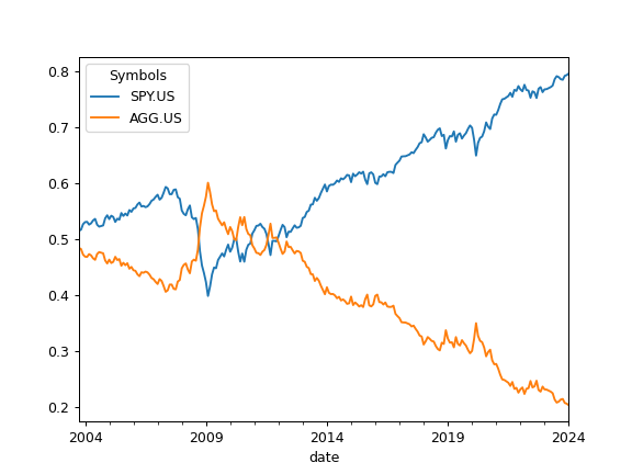
- property weights_ts
Calculate assets weights time series considering rebalancing strategy.
The weights of assets in Portfolio are not constant if rebalancing_period is different from ‘month’.
- Returns:
- DataFrame
Weights of assets time series.
Examples
>>> import matplotlib.pyplot as plt
>>> reb_period = ok.Rebalance(period="none")  # The Portfolio is not rebalanced.
>>> pf = ok.Portfolio(["SPY.US", "AGG.US"], weights=[0.5, 0.5], rebalancing_strategy=reb_period)
>>> pf.weights_ts.plot()
>>> plt.show()
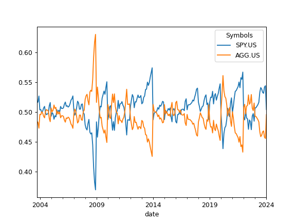
The weights of assets time series will differ significantly if the portfolio rebalancing_period is 1 year.
>>> pf.rebalancing_strategy = ok.Rebalance(period="year")  # set a new rebalancing period
>>> pf.weights_ts.plot()
>>> plt.show()
- property rebalancing_events
Time series with the dates of rebalancing events.
Each event has the type of rebalancing event: - calendar (calendar event) - abs (rebalancing by absolute deviation) - rel (rebalancing by relative deviation)
- Returns:
- DataFrame
Dates of rebalancing events time series.
Examples
>>> pf = ok.Portfolio(
...     assets=["SPY.US", "AGG.US"],
...     weights=[0.5, 0.5],
...     rebalancing_strategy=ok.Rebalance(period="year", abs_deviation=0.05),
... )
>>> pf.rebalancing_events
date
2004-05    calendar
2005-05    calendar
2006-05    calendar
2007-05    calendar
2008-05    calendar
             ...
2020-05    calendar
2020-11         abs
2021-05    calendar
2022-05    calendar
2023-05    calendar
Name: event, Length: 21, dtype: object
- property rebalancing_strategy
Return rebalancing strategy of the portfolio.
Rebalancing is the process by which an investor restores their portfolio to its target allocation by selling and buying assets. After rebalancing all the assets have original weights.
Rebalancing period (rebalancing frequency) is predetermined time intervals when the investor rebalances the portfolio.
- Returns:
- Rebalance
Portfolio rebalancing strategy.
Examples
>>> pf = ok.Portfolio(
...     assets=["SPY.US", "AGG.US"],
...     weights=[0.5, 0.5],
...     rebalancing_strategy=ok.Rebalance(period="year", abs_deviation=0.05),
... )
>>> pf.rebalancing_strategy
Rebalance(period='year', abs_deviation=0.05, rel_deviation=None)
- property symbol
Return a text symbol of portfolio.
Symbols are similar to tickers but have a namespace information:
SPY.US is a symbol
SPY is a ticker
Portfolios have ‘.PF’ as a namespace.
- Returns:
- str
Text symbol of the portfolio.
Examples
>>> p = ok.Portfolio()
>>> p.symbol  # a randomly generated symbol will be shown
'portfolio_5312.PF'
>>> p.symbol = "spy_portfolo.PF" # The symbol can be customized after initialization
New Portfolio can have a custom symbol.
>>> p = ok.Portfolio(symbol="aggressive.PF")
>>> p.symbol
'aggressive.PF'
- property name
Return text name of portfolio.
For Portfolio name is equal to symbol.
- Returns:
- str
Text name of the portfolio.
>>> p = ok.Portfolio()
    ..
>>> p.name
    ..
- ‘portfolio_5312.PF’
- property ror
Calculate monthly rate of return time series for portfolio considering rebalancing strategy.
- Returns:
- Series
Rate of return monthly time series for the portfolio.
Examples
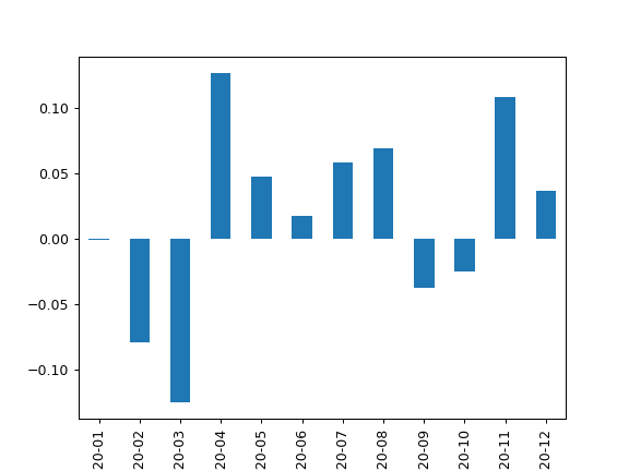
>>> pf = ok.Portfolio(first_date="2020-01", last_date="2020-12")
>>> pf.ror
Date
2020-01   -0.0004
2020-02   -0.0792
2020-03   -0.1249
2020-04    0.1270
2020-05    0.0476
2020-06    0.0177
2020-07    0.0589
2020-08    0.0698
2020-09   -0.0374
2020-10   -0.0249
2020-11    0.1088
2020-12    0.0370
Freq: M, Name: portfolio_4669.PF, dtype: float64
>>> import matplotlib.pyplot as plt
>>> pf.ror.plot(kind="bar")
>>> plt.show()
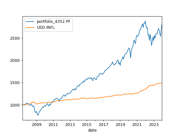
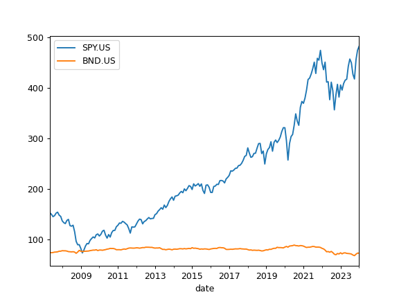
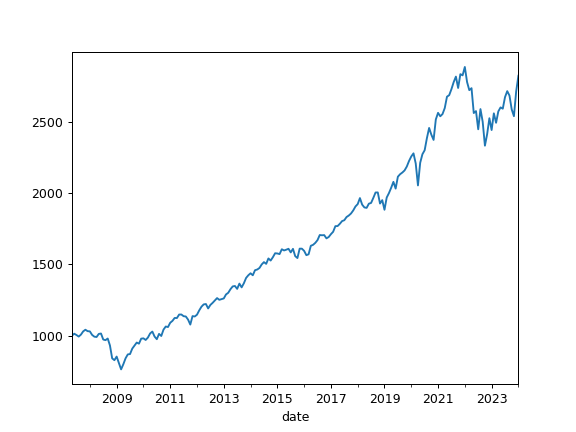
- property wealth_index
Calculate wealth index time series for the portfolio and accumulated inflation.
Wealth index (Cumulative Wealth Index) is a time series that presents the value of portfolio over historical time period. Accumulated inflation time series is added if inflation=True in the Portfolio.
Wealth index is obtained from the accumulated return multiplied by the initial investments. That is: 1000 * (Acc_Return + 1) Initial investments are taken as 1000 units of the Portfolio base currency.
- Returns:
- DataFrame
Time series of wealth index values for portfolio and accumulated inflation.
Examples
>>> import matplotlib.pyplot as plt
>>> x = ok.Portfolio(["SPY.US", "BND.US"])
>>> x.wealth_index.plot()
>>> plt.show()
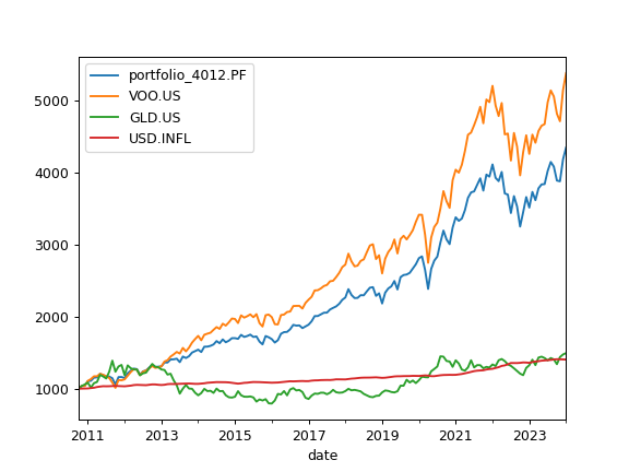
- property wealth_index_with_assets
Calculate wealth index time series for the portfolio, all assets and accumulated inflation.
Cash flows are not taken into account.
Wealth index (Cumulative Wealth Index) is a time series that presents the value of portfolio over historical time period. Accumulated inflation time series is added if inflation=True in the Portfolio.
Wealth index is obtained from the accumulated return multiplied by the initial investments. initial_amount_pv * (Acc_Return + 1)
- Returns:
- DataFrame
Time series of wealth index values for portfolio, each asset and accumulated inflation.
Examples
>>> import matplotlib.pyplot as plt
>>> pf = ok.Portfolio(["VOO.US", "GLD.US"], weights=[0.8, 0.2])
>>> pf.wealth_index_with_assets.plot()
>>> plt.show()
- property mean_return_monthly
Calculate monthly mean return (arithmetic mean) for the portfolio rate of return time series.
Mean return calculated for the full history period.
- Returns:
- float
Mean return value.
Examples
>>> pf = ok.Portfolio(["ISF.LSE", "XGLE.LSE"], weights=[0.6, 0.4], ccy="GBP")
>>> pf.mean_return_monthly
0.0001803312727272665
- property mean_return_annual
Calculate annualized mean return (arithmetic mean) for the portfolio rate of return time series.
Mean return calculated for the full history period.
- Returns:
- float
Mean return value.
Examples
>>> pf = ok.Portfolio(["XCS6.XETR", "PHAU.LSE"], weights=[0.85, 0.15], ccy="USD")
>>> pf.names
{'XCS6.XETR': 'Xtrackers MSCI China UCITS ETF 1C', 'PHAU.LSE': 'WisdomTree Physical Gold'}
>>> pf.mean_return_annual
0.09005826844072184
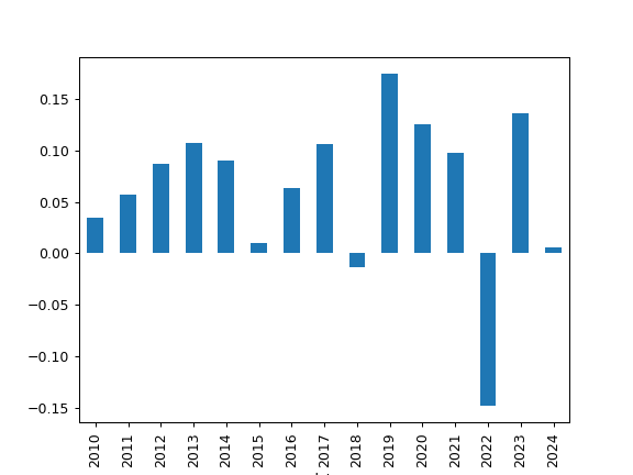
- annual_return_ts(return_type='cagr')
Calculate annual rate of return time series for portfolio.
Rate of return is calculated for each calendar year.
- Parameters:
- return_type{‘cagr’, ‘arithmetic_mean’}, default ‘cagr’
Method used to calculate annual returns.
- Returns:
- Series
Calendar annual rate of return time series.
Examples
>>> import matplotlib.pyplot as plt
>>> pf = ok.Portfolio(["VOO.US", "AGG.US"], weights=[0.4, 0.6])
>>> pf.annual_return_ts().plot(kind="bar")
>>> plt.show()
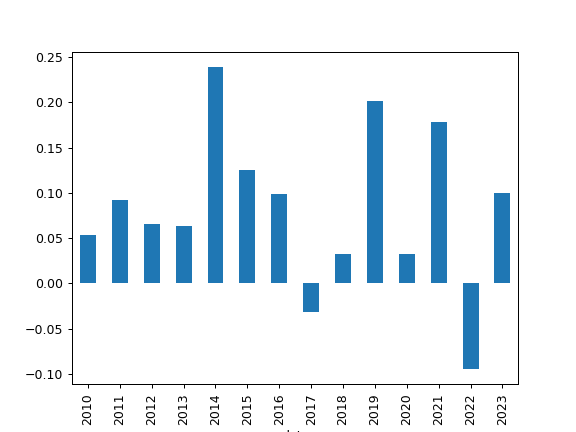
Plot annual returns for portfolio with EUR as the base currency.
>>> pf = ok.Portfolio(["VOO.US", "AGG.US"], weights=[0.4, 0.6], ccy="EUR")
>>> pf.annual_return_ts().plot(kind="bar")
>>> plt.show()
- get_cagr(period=None, real=False)
Calculate the expanding portfolio Compound Annual Growth Rate (CAGR) time series.
The expanding CAGR at each month is the annualized rate of return required for the investment to grow from its initial value to its value at that month, assuming all incomes were reinvested. The last row contains the CAGR over the full selected period.
Inflation adjusted annualized returns (real CAGR) are shown with real=True option. Annualized inflation is calculated for the same period if inflation=True in the Portfolio.
- Parameters:
- periodint, default None
CAGR trailing period in years. If None, use the full available period.
- realbool, default False
CAGR is adjusted for inflation (real CAGR) if True. Portfolio should be initiated with inflation=True for real CAGR.
- Returns:
- DataFrame
Time series of expanding portfolio CAGR and annualized inflation (if inflation=True in Portfolio and real=False).
Notes
CAGR is not defined for periods less than 1 year. The first 11 rows are filled with NaN values.
Examples
>>> pf = ok.Portfolio(["SPY.US", "BND.US"], weights=[0.6, 0.4], ccy="USD", inflation=True)
>>> pf.get_cagr(period=5).tail()
The last row contains the CAGR values over the full selected period.
To get inflation adjusted annualized return (real CAGR) add real=True option:
>>> pf.get_cagr(period=5, real=True).tail()
- get_rolling_cagr(window=12, real=False)
Calculate rolling CAGR (Compound Annual Growth Rate) for the portfolio.
- Parameters:
- windowint, default 12
Size of the moving window in months. Window size should be at least 12 months for CAGR.
- realbool, default False
CAGR is adjusted for inflation (real CAGR) if True. Portfolio should be initiated with Inflation=True for real CAGR.
- Returns:
- DataFrame
Time series of rolling CAGR and mean inflation (optionally).
Notes
CAGR is not defined for periods less than 1 year (NaN values are returned).
Examples
>>> x = ok.Portfolio(["SPY.US", "BND.US"], ccy="EUR", inflation=True)
>>> x.get_rolling_cagr(window=5 * 12, real=True)
         portfolio_...
date
...             ...
- get_monthly_geometric_mean_return()
Calculate monthly geometric mean return for the portfolio.
The geometric mean return is the constant periodic return that would produce the same final value as a sequence of varying periodic returns when compounded over time.
- Returns:
- float
Monthly geometric mean return value.
Examples
>>> pf = ok.Portfolio(["SPY.US", "AGG.US"], weights=[0.6, 0.4])
>>> pf.get_monthly_geometric_mean_return()
0.005321
- get_cumulative_return(period=None, real=False)
Calculate the expanding cumulative return time series for the portfolio.
The cumulative return is the total compounded change in the portfolio price from the start of the selected period up to and including each subsequent month. The last row contains the cumulative return over the full selected period.
Inflation adjusted cumulative returns (real cumulative returns) are shown with real=True option. Inflation data is taken from the same period if inflation=True in the Portfolio.
- Parameters:
- periodstr or int or None, default None
Trailing period in years. None - full time cumulative return. ‘YTD’ - (Year To Date) period of time beginning the first day of the calendar year up to the last month.
- realbool, default False
Cumulative return is adjusted for inflation (real cumulative return) if True. Portfolio should be initiated with Inflation=True for real cumulative return.
- Returns:
- DataFrame
Time series of cumulative return for the portfolio and cumulative inflation (if inflation=True in Portfolio and real=False).
Examples
>>> pf = ok.Portfolio(["BTC-USD.CC", "LTC-USD.CC"], weights=[0.8, 0.2], last_date="2021-03")
>>> pf.get_cumulative_return(period=2, real=True).tail()
         portfolio_6232.PF
2020-11           3.624500
2020-12           5.125700
2021-01           7.328400
2021-02           8.612000
2021-03           9.393810
The last row contains the cumulative return over the full selected period.
- get_rolling_cumulative_return(window=12, real=False)
Calculate rolling cumulative return.
The cumulative return is the total change in the portfolio price.
- Parameters:
- windowint, default 12
Size of the moving window in months.
- realbool, default False
Cumulative return is adjusted for inflation (real cumulative return) if True. Portfolio should be initiated with Inflation=True for real cumulative return.
- Returns:
- DataFrame
Time series of rolling cumulative return and inflation (optional).
Examples
>>> pf = ok.Portfolio(
...     ["SPY.US", "AGG.US", "GLD.US"],
...     weights=[0.6, 0.35, 0.05],
...     rebalancing_strategy=ok.Rebalance(period="year"),
... )
>>> pf.get_rolling_cumulative_return(window=24, real=True)
         portfolio_9012.PF
2006-11           0.125728
2006-12           0.104348
2007-01           0.129601
2007-02           0.110680
2007-03           0.132610
                    ...
2021-03           0.263755
2021-04           0.275474
2021-05           0.322736
2021-06           0.264963
2021-07           0.273801
[177 rows x 1 columns]
- property close_monthly
Portfolio size monthly time series.
Portfolio size is shown in base currency units. It is similar to the close value of an asset. Initial portfolio value is equal to 1000 units of base currency.
- Returns:
- pd.Series
Monthly portfolio size time series.
Notes
‘close_mothly’ shows the same output as the ‘wealth_index’. This property is required as Portfolio must have the same attributes as an Asset.
Examples
>>> import matplotlib.pyplot as plt
>>> pf = ok.Portfolio(["SPY.US", "BND.US"], ccy="USD")
>>> pf.close_monthly.plot()
>>> plt.show()
- property number_of_securities
Calculate the number of securities monthly time series for the portfolio assets.
The number of securities in the Portfolio is changing over time as the dividends are reinvested. Portfolio rebalancing also affects the number of securities.
Initial number of securities depends on the portfolio size in base currency (1000 units).
- Returns:
- DataFrame
Number of securities monthly time series for the portfolio assets.
Examples
>>> pf = ok.Portfolio(["SPY.US", "BND.US"], ccy="USD", last_date="07-2021")
>>> pf.number_of_securities
           SPY.US     BND.US
Date
2007-05  3.261153   6.687174
2007-06  3.337216   6.758447
2007-07  3.407015   6.643519
2007-08  3.410268   6.663862
2007-09  3.372630   6.798730
           ...        ...
2021-03  3.273521  15.313911
2021-04  3.204779  15.685601
2021-05  3.196768  15.749127
2021-06  3.186124  15.879056
2021-07  3.166335  16.003569
[171 rows x 2 columns]
- property dividends
Calculate portfolio dividends monthly time series.
Portfolio dividends are obtained by summing asset dividends adjusted to the base currency. Dividends size depends on the portfolio value and number of securities.
- Returns:
- Series
Portfolio dividends monthly time series.
Examples
>>> pf = ok.Portfolio(["SPY.US", "BND.US"], ccy="USD", last_date="07-2021")
>>> pf.dividends
2007-05    0.849271
2007-06    3.928855
2007-07    1.551262
2007-08    2.023148
2007-09    4.423416
             ...
2021-03    6.155337
2021-04    3.019478
2021-05    2.056836
2021-06    6.519521
2021-07    2.114071
Freq: M, Name: portfolio_2951.PF, Length: 171, dtype: float64
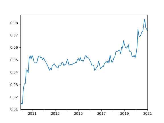
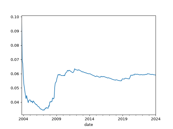
- property dividend_yield
Calculate last twelve months (LTM) dividend yield time series for the portfolio. Time series has monthly values.
Portfolio dividend yield is a weighted sum of the assets dividend yields (adjusted to the portfolio base currency).
For an asset LTM dividend yield is the sum trailing twelve months of common dividends per share divided by the current price per share.
- Returns:
- Series
Portfolio LTM dividend yield monthly time series.
Examples
>>> pf = ok.Portfolio(["T.US", "XOM.US"], weights=[0.8, 0.2], first_date="2010-01", last_date="2021-01", ccy="USD")
>>> pf.dividend_yield
2010-01    0.013249
2010-02    0.014835
2010-03    0.014257
             ...
2020-11    0.076132
2020-12    0.074743
2021-01    0.073643
Freq: M, Name: portfolio_8836.PF, Length: 133, dtype: float64
>>> import matplotlib.pyplot as plt
>>> pf.dividend_yield.plot()
>>> plt.show()
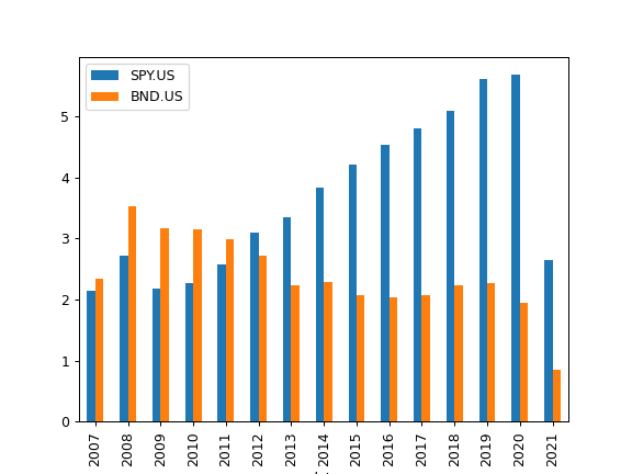
- property dividends_annual
Return calendar year dividends sum time series for each asset.
- Returns:
- DataFrame
Annual dividends time series for each asset.
Examples
>>> import matplotlib.pyplot as plt
>>> pf = ok.Portfolio(["SPY.US", "BND.US"], ccy="USD", last_date="07-2021")
>>> pf.dividends_annual.plot(kind="bar")
>>> plt.show()
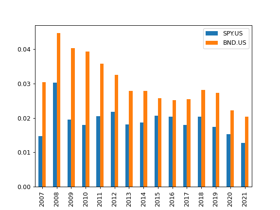
- property dividend_yield_annual
Calculate last twelve months (LTM) dividend yield annual time series.
Time series is based on the dividend yield for the end of calendar year.
LTM dividend yield is the sum trailing twelve months of common dividends per share divided by the current price per share.
All yields are calculated in the asset list base currency after adjusting the dividends and price time series. Forecasted (future) dividends are removed.
- Returns:
- DataFrame
Time series of LTM dividend yield for each asset.
See also
dividend_yieldDividend yield time series.
dividends_annualCalendar year dividends time series.
dividend_paying_yearsNumber of years of consecutive dividend payments.
dividend_growing_yearsNumber of years when the annual dividend was growing.
get_dividend_mean_yieldArithmetic mean for annual dividend yield.
get_dividend_mean_growth_rateGeometric mean of annual dividends growth rate.
Examples
>>> import matplotlib.pyplot as plt
>>> pf = ok.Portfolio(["SPY.US", "BND.US"], ccy="USD", last_date="07-2021")
>>> pf.dividend_yield_annual.plot(kind="bar")
>>> plt.show()
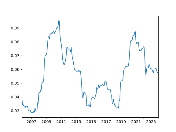
- property assets_dividend_yield
Calculate last twelve months (LTM) dividend yield time series (monthly) for each asset.
LTM dividend yield is the sum trailing twelve months of common dividends per share divided by the current price per share.
All yields are calculated in the asset list base currency after adjusting the dividends and price time series. Forecasted (future) dividends are removed. Zero value time series are created for assets without dividends.
- Returns:
- DataFrame
Monthly time series of LTM dividend yield for each asset.
See also
dividend_yield_annualCalendar year dividend yield time series.
dividends_annualCalendar year dividends time series.
dividend_paying_yearsNumber of years of consecutive dividend payments.
dividend_growing_yearsNumber of years when the annual dividend was growing.
get_dividend_mean_yieldArithmetic mean for annual dividend yield.
get_dividend_mean_growth_rateGeometric mean of annual dividends growth rate.
Examples
>>> x = ok.AssetList(["T.US", "XOM.US"], first_date="1984-01", last_date="1994-12")
>>> x.dividend_yield
           T.US    XOM.US
1984-01  0.000000  0.000000
1984-02  0.000000  0.002597
1984-03  0.002038  0.002589
1984-04  0.001961  0.002346
           ...       ...
1994-09  0.018165  0.012522
1994-10  0.018651  0.011451
1994-11  0.018876  0.012050
1994-12  0.019344  0.011975
[132 rows x 2 columns]
- property real_mean_return
Calculate annualized real mean return (arithmetic mean) for the rate of return time series.
Real rate of return is adjusted for inflation. Real return is defined if there is an inflation=True option in Portfolio.
- Returns:
- float
Annualized value of the mean for the real rate of return time series.
Examples
>>> pf = ok.Portfolio(["MSFT.US", "AAPL.US"])
>>> pf.real_mean_return
0.3088967455111862
- property risk_monthly
Calculate monthly risk expanding time series for Portfolio.
Monthly risk of portfolio is a standard deviation of the rate of return time series. Standard deviation (sigma) is normalized by N-1.
- Returns:
- Series
Standard deviation of the monthly return expanding time series.
See also
risk_annualCalculate annualized risks.
semideviation_monthlyCalculate semideviation monthly values.
semideviation_annualCalculate semideviation annualized values.
get_var_historicCalculate historic Value at Risk (VaR).
get_cvar_historicCalculate historic Conditional Value at Risk (CVaR).
drawdownsCalculate drawdowns.
Examples
>>> pf = ok.Portfolio(["MSFT.US", "AAPL.US"])
>>> pf.risk_monthly
date
1986-05    0.020117
1986-06    0.122032
1986-07    0.130113
1986-08    0.116642
             ...
2023-08    0.092875
2023-09    0.092861
2023-10    0.092759
2023-11    0.092763
2023-12    0.092665
Freq: M, Name: portfolio_1094.PF, Length: 453, dtype: float64
- property risk_annual
Calculate annualized risk expanding time series for portfolio.
Risk is a standard deviation of the rate of return.
Annualized risk is calculated for rate of retirun time series for the sample from ‘first_date’ to ‘last_date’.
- Returns:
- Series
Annualized standard deviation of the monthly return expanding time series.
Examples
>>> pf = ok.Portfolio(["MSFT.US", "AAPL.US"])
>>> pf.risk_annual
date
1986-05    0.285175
1986-06    0.890909
1986-07    0.616876
1986-08    0.632270
1986-09    0.509642
             ...
2023-08    0.428297
2023-09    0.427350
2023-10    0.426961
2023-11    0.427930
- property semideviation_monthly
Calculate semi-deviation monthly value for portfolio rate of return time series.
Semi-deviation (Downside risk) is the risk of the return being below the expected return.
- Returns:
- float
Semi-deviation monthly value for portfolio rate of return time series.
Examples
>>> pf = ok.Portfolio(["MSFT.US", "AAPL.US"], last_date="2024-12")
>>> pf.semideviation_monthly
0.057319735856567695
- property semideviation_annual
Return semideviation annualized value for portfolio rate of return time series.
Semi-deviation (Downside risk) is the risk of the return being below the expected return.
- Returns:
- float
Annualized semi-deviation monthly value for portfolio rate of return time series.
Examples
>>> pf = ok.Portfolio(["MSFT.US", "AAPL.US"], last_date="2024-12")
>>> pf.semideviation_annual
0.1985613895600056
- get_var_historic(time_frame=12, level=1)
Calculate historic Value at Risk (VaR) for the portfolio.
The VaR calculates the potential loss of an investment with a given time frame and confidence level. Loss is a positive number (expressed in cumulative return). If VaR is negative there are expected gains at this confidence level.
- Parameters:
- time_frameint, default 12
Time frame for VAR. Default is 12 months.
- levelint, default 1
Confidence level in percents. Default value is 1%.
- Returns:
- float
Historic Value at Risk (VaR) value for the portfolio.
Examples
>>> x = ok.Portfolio(["SP500TR.INDX", "SP500BDT.INDX"], last_date="2021-01")
>>> x.get_var_historic(time_frame=12, level=1)
0.24030006476701732
- get_cvar_historic(time_frame=12, level=1)
Calculate historic Conditional Value at Risk (CVAR, expected shortfall) for the portfolio.
CVaR is the average loss over a specified time period of unlikely scenarios beyond the confidence level. Loss is a positive number (expressed in cumulative return). If CVaR is negative there are expected gains at this confidence level.
- Parameters:
- time_frameint, default 12
Time period size in months.
- levelint, default 1
Confidence level in percents to calculate the VaR. Default value is 1% (1% quantile).
- Returns:
- float
Historic Conditional Value at Risk (CVAR, expected shortfall) value for the portfolio.
Examples
>>> x = ok.Portfolio(["USDEUR.FX", "BTC-USD.CC"], last_date="2021-01")
>>> x.get_cvar_historic(time_frame=2, level=1)
0.3566909250442616
- property drawdowns
Calculate drawdowns time series for the portfolio.
The drawdown is the percent decline from a previous peak in wealth index.
- Returns:
- Series
Drawdowns time series for the portfolio
- property real_drawdowns
Calculate real (inflation-adjusted) drawdowns time series for the portfolio.
The real drawdown is the percent decline from a previous peak in the inflation-adjusted wealth index. Portfolio should be initiated with inflation=True for real drawdowns.
- Returns:
- Series
Real drawdowns time series for the portfolio.
See also
drawdownsCalculate drawdowns (not adjusted for inflation).
Examples
>>> import matplotlib.pyplot as plt
>>> pf = ok.Portfolio(["SPY.US", "BND.US"], inflation=True, last_date="2021-08")
>>> pf.real_drawdowns.plot()
>>> plt.show()
- property price_drawdowns
Calculate price drawdowns time series for the portfolio.
The price drawdown is the percent decline from a previous peak in the portfolio price index. The price index is built from the assets close prices (not adjusted for dividends) with the same weights and rebalancing strategy as the portfolio, hence price drawdowns may significantly differ from drawdowns (based on total return) for portfolios with high dividend assets.
The price index is anchored at the first month of the period, so price drawdowns cover the same months as drawdowns.
- Returns:
- Series
Price drawdowns time series for the portfolio.
See also
drawdownsCalculate drawdowns from total return (with dividends reinvested).
Examples
>>> import matplotlib.pyplot as plt
>>> pf = ok.Portfolio(["SPY.US", "BND.US"], ccy="USD", last_date="2021-08")
>>> pf.price_drawdowns.plot()
>>> plt.show()
- property recovery_period
Get recovery period time series for the portfolio value.
The recovery period (drawdown duration) is the number of months to reach the value of the last maximum.
- Returns:
- pd.Series
Recovery period time series for the portfolio value
See also
drawdownsCalculate drawdowns time series.
Notes
The largest recovery period does not necessary correspond to the max drawdown.
Examples
>>> pf = ok.Portfolio(["SPY.US", "AGG.US"], weights=[0.5, 0.5])
>>> pf.recovery_period.nlargest()
date
2010-10    35
2004-10     7
2012-01     7
2019-03     6
2018-07     5
Freq: M, Name: portfolio_5724.PF, dtype: int32
- describe(years=(1, 5, 10))
Generate descriptive statistics for the portfolio.
Statistics includes:
YTD (Year To date) compound return
CAGR for a given list of periods and full available period
Annualized mean rate of return (full available period)
LTM Dividend yield - last twelve months dividend yield
Risk metrics (full available period):
risk (standard deviation)
CVAR (timeframe is 1 year)
max drawdowns (and dates)
- Parameters:
- yearstuple of int, default (1, 5, 10)
List of periods for CAGR statistics.
- Returns:
- DataFrame
Table of descriptive statistics for the portfolio.
See also
get_cumulative_returnCalculate cumulative return.
get_cagrCalculate portfolio Compound Annual Growth Rate (CAGR).
dividend_yieldCalculate dividend yield (LTM).
risk_annualReturn annualized risks (standard deviation).
get_cvar_historicCalculate historic Conditional Value at Risk (CVAR, expected shortfall).
drawdownsCalculate drawdowns.
Examples
>>> pf = ok.Portfolio(["SPY.US", "BND.US"], ccy="USD", last_date="07-2021")
>>> pf.describe(years=[2, 5, 7])  # 'years' customizes the timeframe for the CAGR
            property              period portfolio_2951.PF  inflation
0    compound return                 YTD          0.084098   0.048154
1               CAGR             2 years          0.141465   0.031566
2               CAGR             5 years          0.102494   0.025582
3               CAGR             7 years          0.091694   0.019656
4               CAGR  14 years, 3 months          0.074305   0.019724
5     Dividend yield                 LTM          0.016504        NaN
6               Risk  14 years, 3 months          0.086103        NaN
7               CVAR  14 years, 3 months          0.214207        NaN
8       Max drawdown  14 years, 3 months         -0.266915        NaN
9  Max drawdown date  14 years, 3 months           2009-02        NaN
- property table
Return table with security name, ticker, weight for assets in the portfolio.
When at least one asset has a local name, an additional ‘local name’ column is inserted between ‘asset name’ and ‘ticker’.
- Returns:
- DataFrame
Security name - ticker - weight table.
Examples
>>> pf = ok.Portfolio(["MSFT.US", "AAPL.US"])
>>> pf.table
                asset name   ticker  weights
0  Microsoft Corporation  MSFT.US      0.5
1              Apple Inc  AAPL.US      0.5
>>> pf = ok.Portfolio(["SBER.MOEX", "MSFT.US"])
>>> pf.table
              asset name             local name     ticker  weights
0               Sberbank               Сбербанк  SBER.MOEX      0.5
1  Microsoft Corporation  Microsoft Corporation    MSFT.US      0.5
- percentile_inverse_cagr(years=1, score=0)
Compute the percentile rank of a score (CAGR value).
Percentile rank can be calculated for a historical distribution of CAGR.
If percentile_inverse of, for example, 0% (CAGR value) is equal to 8% for 1 year time frame it means that 8% of the CAGR values in the distribution are negative in 1 year periods. Or in other words the probability of getting negative result after 1 year of investments is 8%.
- Parameters:
- yearsint, default 1
Period length (time frame) in years when CAGR is calculated.
- scorefloat, default 0
Score that is compared to the elements in CAGR array.
- Returns:
- float
Percentile-position of score (0-100) relative to distribution.
Examples
>>> pf = ok.Portfolio(
...     ["SPY.US", "AGG.US", "GLD.US"],
...     weights=[0.60, 0.35, 0.05],
...     rebalancing_strategy=ok.Rebalance(period="year"),
... )
>>> pf.percentile_inverse_cagr(score=0, years=1)
18.08
The probability of getting negative result (score=0) in 1 year period for historical distribution.
- property assets_close_monthly
Show assets monthly close time series adjusted to the base currency.
- Returns:
- DataFrame
Assets monthly close time series adjusted to the base currency.
Examples
>>> import matplotlib.pyplot as plt
>>> al = ok.AssetList(["SPY.US", "BND.US"], ccy="USD")
>>> al.assets_close_monthly.plot()
>>> plt.show()
- property assets_ror
Rate of return monthly time series for all assets.
- Returns:
- DataFrame
Rate of return monthly data.
- property currency
Return the base currency.
Such properties as rate of return and risk are adjusted to the base currency.
- Returns:
- str
Base currency.
- percentile_cagr(years, percentiles=[10, 50, 90])
Calculate given percentiles for portfolio rolling CAGR distribution from the historical data.
CAGR - Compound Annual Growth Rate. Each percentile is calculated for a period range from 1 year to ‘years’.
- Parameters:
- yearsint
Max window size for rolling CAGR in the distribution in years. It should not exceed 1/2 of the portfolio history period length ‘period_length’.
- percentileslist of int, default [10, 50, 90]
List of percentiles to be calculated.
- Returns:
- DataFrame
Table with percentiles values for each period from 1 to ‘years’.
Examples
>>> pf = ok.Portfolio(
...     ["SPY.US", "AGG.US", "GLD.US"],
...     weights=[0.60, 0.35, 0.05],
...     rebalancing_strategy=ok.Rebalance(period="none"),
... )
>>> pf.percentile_cagr(years=5, percentiles=[1, 50, 99])
             1         50        99
years
1     -0.231327  0.098693  0.295343
2     -0.101689  0.091824  0.206471
3     -0.036771  0.085428  0.157833
4     -0.007674  0.085178  0.142195
5      0.030933  0.082865  0.134496
- plot_assets(kind='mean', tickers='tickers', pct_values=False, xy_text=(0, 10), **kwargs)
Plot asset points on the risk-return chart with annotations.
Annualized values for risk and return are used. Risk is the standard deviation of monthly rate of return time series. Return can be an annualized mean return (expected return) or CAGR (compound annual growth rate).
- Parameters:
- kind{‘mean’, ‘cagr’}, default ‘mean’
Type of return: annualized mean return (expected return) or CAGR (compound annual growth rate).
- tickers{‘tickers’, ‘names’, ‘local_names’} or list of str, default ‘tickers’
Annotation type for assets.
‘tickers’: asset symbols are shown in the form ‘SPY.US’.
‘names’: asset names are shown (for example, ‘SPDR S&P 500 ETF Trust’).
‘local_names’: native-language names (e.g. ‘Сбербанк’ / ‘贵州茅台’).
list of str: custom annotations for each asset.
Note
Rendering native (‘local_names’) labels written in CJK scripts (Chinese, Japanese, Korean) requires a CJK-capable matplotlib font; with the default fonts such glyphs appear as tofu boxes.
- pct_valuesbool, default False
If True, show risk and return values in percent. If False, show values as decimals.
- xy_texttuple, default (0, 10)
The shift of the annotation text (x, y) from the point.
- **kwargs
Arbitrary keyword arguments passed to matplotlib.pyplot.scatter.
- Returns:
- Axes
Matplotlib axes object.
Examples
>>> import matplotlib.pyplot as plt
>>> al = ok.AssetList(["SPY.US", "AGG.US"], ccy="USD", inflation=False)
>>> al.plot_assets()
>>> plt.show()
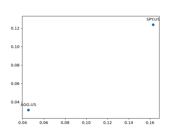
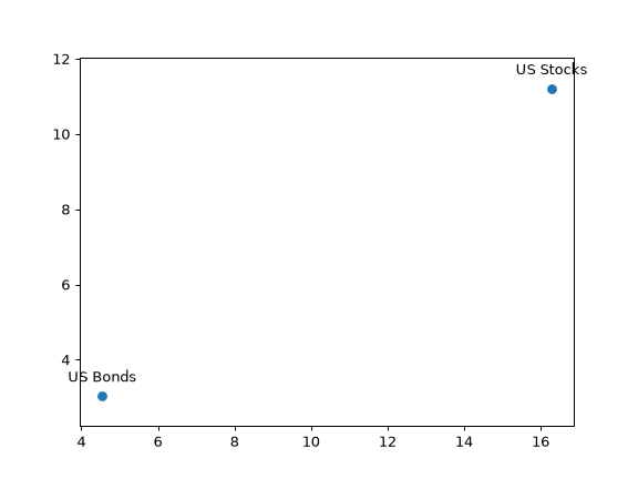
Plotting with default parameters values shows expected return, ticker annotations and algebraic values for risk and return. To use CAGR instead of expected return use kind=’cagr’.
>>> al.plot_assets(
...     kind="cagr",
...     tickers=["US Stocks", "US Bonds"],  # use custom annotations for the assets
...     pct_values=True,  # risk and return values are in percents
... )
>>> plt.show()
- property symbols
Return a list of used financial symbols.
Symbols are similar to tickers but have a namespace information:
SPY.US is a symbol
SPY is a ticker
- Returns:
- list of str
List of used symbols.
- property tickers
Return a list of used tickers (symbols without a namespace).
Tickers are similar to symbols but do not have namespace information:
SPY is a ticker
SPY.US is a symbol
- Returns:
- list of str
List of used tickers.
- get_sharpe_ratio(rf_return=0)
Calculate Sharpe ratio.
The Sharpe ratio is the average annual return in excess of the risk-free rate per unit of risk (annualized standard deviation).
Risk-free rate should be taken according to the Portfolio base currency.
- Parameters:
- rf_returnfloat, default 0
Risk-free rate of return.
- Returns:
- float
Examples
>>> pf = ok.Portfolio(["VOO.US", "BND.US"], weights=[0.40, 0.60])
>>> pf.get_sharpe_ratio(rf_return=0.04)
0.7412193684695373
- get_sortino_ratio(t_return=0)
Calculate Sortino ratio for the portfolio with specified target return.
Sortion ratio measures the risk-adjusted return of portfolio. It is a modification of the Sharpe ratio but penalizes only those returns falling below a specified target rate of return, while the Sharpe ratio penalizes both upside and downside volatility equally.
- Parameters:
- t_returnfloat, default 0
Traget rate of return.
- Returns:
- float
Examples
>>> pf = ok.Portfolio(["VOO.US", "BND.US"], last_date="2021-12")
>>> pf.get_sortino_ratio(t_return=0.02)
1.4377728903230174
- tracking_error(benchmark, rolling_window=None, method='rms')
Calculate ex-post tracking error time series of the portfolio against a benchmark.
Tracking error is an ex-post (backward-looking) measure of how closely the portfolio follows the benchmark. It is computed from the realized monthly return differences between the portfolio and the benchmark, and is annualized (multiplied by sqrt(12)). Tracking error values are decimal fractions: 0.05 corresponds to 5% annualized.
Two formulas are available (method parameter):
“rms” (default): root-mean-square of the return differences. The differences are not centered around their mean, hence the systematic lag between the portfolio and the benchmark (tracking difference) is included in the result.
“std”: sample standard deviation of the return differences with Bessel’s correction — the classic tracking error definition (Hwang & Satchell, “Tracking Error: Ex-Ante versus Ex-Post Measures”, 2001, eq. 2) measuring the pure volatility of deviations from the benchmark. The first point of the expanding time series is dropped (a single observation has no standard deviation).
The benchmark rate of return is converted to the portfolio base currency, and the time period is limited to the intersection of the portfolio and benchmark available histories.
- Parameters:
- benchmarkstr, Asset, Portfolio
Benchmark ticker (e.g. “SP500TR.INDX”) or an asset-like object (Asset, Portfolio).
- rolling_windowint or None, default None
Size of the moving window in months. Must be at least 12 months. If None calculate expanding tracking error.
- method{“rms”, “std”}, default “rms”
Tracking error formula: “rms” for the uncentered root-mean-square of return differences, “std” for the centered sample standard deviation.
- Returns:
- Series
Expanding or rolling annualized tracking error time series. The series is named after the portfolio symbol.
Examples
>>> import matplotlib.pyplot as plt
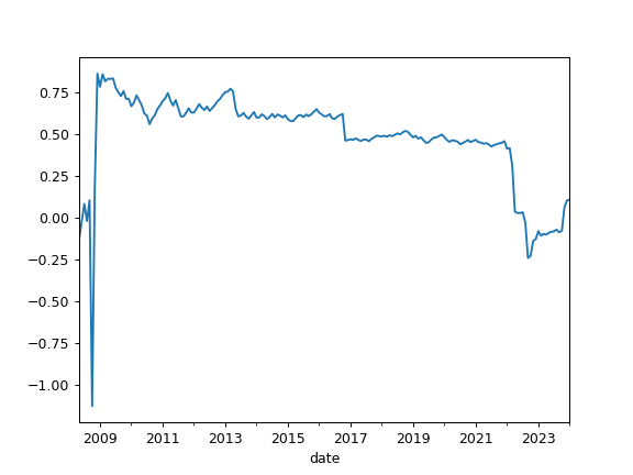
>>> pf = ok.Portfolio(["SPY.US", "AGG.US"], weights=[0.60, 0.40], last_date="2024-01")
>>> pf.tracking_error(benchmark="SP500TR.INDX").plot()
>>> plt.show()
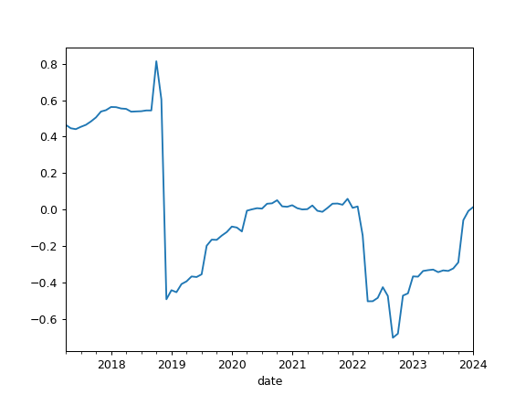
To calculate rolling tracking error set rolling_window to a number of months (moving window size):
>>> pf.tracking_error(benchmark="SP500TR.INDX", rolling_window=24, method="std").plot()
>>> plt.show()
- property diversification_ratio
Calculate Diversification Ratio for the portfolio.
The Diversification Ratio is the ratio of the weighted average of assets risks divided by the portfolio risk. In this case risk is the annuilized standatd deviation for the rate of return .
- Returns:
- float
Examples
>>> pf = ok.Portfolio(["VOO.US", "BND.US"], weights=[0.7, 0.3], last_date="2021-12")
>>> pf.diversification_ratio
1.1264305597257505
- property okamaio_link
URL link to portfolio at okama.io.
Portfolio with the same tickers, weights and other properties at okama.io financial widgets.
- Returns:
- str
URL link to portfolio at okama.io.
Examples
>>> pf = ok.Portfolio(
...     ["SPY.US", "AGG.US"],
...     weights=[0.60, 0.40],
...     rebalancing_strategy=ok.Rebalance(period="year", abs_deviation=0.05),
... )
>>> pf.okamaio_link
'https://okama.io/portfolio?tickers=SPY.US,AGG.US&ccy=USD&first_date=2003-10&last_date=2024-08&weights=60,40&rebal=year&abs_dev=5&symbol=portfolio_6323.PF'