okama.EfficientFrontier.ef_points

property EfficientFrontier.ef_points

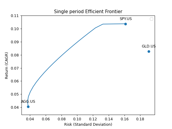
Generate single period Efficient Frontier.

Each point on the Efficient Frontier is a portfolio with optimized risk for a given return.

The points are obtained through the constrained optimization process (optimization with bounds). Bounds are defined with ‘bounds’ property.

Returns:

DataFrame

Table of weights and risk/return values for the Efficient Frontier. The columns:

• assets weights

• CAGR (geometric mean)

• Mean return (arithmetic mean)

• Risk (standard deviation)

All the values are annualized.

Examples

>>> assets = ['SPY.US', 'AGG.US', 'GLD.US']
>>> last_date='2021-07'
>>> y = ok.EfficientFrontier(assets, last_date=last_date)
>>> y.ef_points
        Risk  Mean return      CAGR        AGG.US        GLD.US        SPY.US
0   0.037707     0.041254  0.040579  1.000000e+00  9.278755e-09  2.220446e-16
1   0.036979     0.045042  0.044394  9.473684e-01  0.000000e+00  5.263158e-02
2   0.038027     0.048842  0.048157  8.947368e-01  0.000000e+00  1.052632e-01
3   0.040517     0.052655  0.051879  8.376442e-01  2.061543e-02  1.417404e-01
4   0.043944     0.056481  0.055569  7.801725e-01  4.298194e-02  1.768455e-01
5   0.048125     0.060320  0.059229  7.227015e-01  6.534570e-02  2.119528e-01
6   0.052902     0.064171  0.062856  6.652318e-01  8.770367e-02  2.470646e-01
7   0.058144     0.068035  0.066451  6.077632e-01  1.100558e-01  2.821809e-01
8   0.063753     0.071912  0.070014  5.502956e-01  1.324040e-01  3.173004e-01
9   0.069655     0.075802  0.073543  4.928283e-01  1.547504e-01  3.524213e-01
10  0.075796     0.079704  0.077039  4.353613e-01  1.770958e-01  3.875429e-01
11  0.082136     0.083620  0.080501  3.778987e-01  1.994207e-01  4.226806e-01
12  0.088645     0.087549  0.083928  3.204253e-01  2.217953e-01  4.577794e-01
13  0.095300     0.091491  0.087321  2.629559e-01  2.441514e-01  4.928926e-01
14  0.102084     0.095446  0.090678  2.054869e-01  2.665062e-01  5.280069e-01
15  0.108984     0.099414  0.093999  1.480175e-01  2.888623e-01  5.631202e-01
16  0.115991     0.103395  0.097284  9.054789e-02  3.112196e-01  5.982325e-01
17  0.123096     0.107389  0.100533  3.307805e-02  3.335779e-01  6.333441e-01
18  0.132674     0.111397  0.103452  0.000000e+00  2.432182e-01  7.567818e-01
19  0.161413     0.115418  0.103704  1.110223e-16  1.036379e-09  1.000000e+00

To plot the Efficient Frontier use the DataFrame with the points data. Additionaly ‘Plot.plot_assets()’ can be used to show the assets in the chart.

>>> import matplotlib.pyplot as plt
>>> fig = plt.figure()
>>> # Plot the assets points
>>> y.plot_assets(kind='cagr')  # kind should be set to "cagr" as we take "CAGR" column from the ef_points.
>>> ax = plt.gca()
>>> # Plot the Efficient Frontier
>>> df = y.ef_points
>>> ax.plot(df['Risk'], df['CAGR'])  # we chose to plot CAGR which is geometric mean of return series
>>> # Set the axis labels and the title
>>> ax.set_title('Single period Efficient Frontier')
>>> ax.set_xlabel('Risk (Standard Deviation)')
>>> ax.set_ylabel('Return (CAGR)')
>>> ax.legend()
>>> plt.show()