PortfolioDCF
- class PortfolioDCF(parent, discount_rate=None)
Bases:
objectDiscounted cash flow (DCF) methods for a Portfolio.
This class is available via Portfolio.dcf.
- Parameters:
- parentPortfolio
Parent Portfolio instance.
- discount_ratefloat or None, default None
Annual effective discount rate used to calculate present values (PV). If None and the portfolio has inflation data, the geometric mean of inflation is used. Otherwise, settings.DEFAULT_DISCOUNT_RATE is used.
Examples
>>> pf = ok.Portfolio(first_date="2015-01", last_date="2024-10")
>>> pf.dcf.wealth_index(discounting="fv").head()
Methods & Attributes
cash_flow_ts(discounting[, ...])Cash flow Future Values (FV) or Present Values (PV) time series for the portfolio.
Return the cash flow strategy parameters.
Annual effective discount rate for portfolio cash flow.
find_the_largest_withdrawals_size(goal[, ...])Find the largest withdrawal size for Monte Carlo simulation according to a cash flow strategy.
The future value (FV) of the initial investments at the historical first date.
The discounted value (PV) of the initial investments at the historical first date.
irr()Nominal internal rate of return (money-weighted return, MWRR) of the portfolio cash flow over the full historical period, honoring the configured cash flow strategy.
monte_carlo_cash_flow(discounting[, ...])Calculate portfolio random cash flow (withdrawals/contributions) time series by Monte Carlo simulation.
Distribution of money-weighted IRRs across Monte Carlo forecast paths.
monte_carlo_survival_period([threshold])Generate a survival period distribution for a portfolio with cash flows by Monte Carlo simulation.
monte_carlo_wealth([discounting, ...])Calculate portfolio random wealth indexes with cash flows (withdrawals/contributions) using Monte Carlo simulation.
plot_forecast_monte_carlo([backtest, figsize])Plot Monte Carlo simulation for portfolio future wealth indexes optionally together with historical wealth index.
set_mc_parameters([distribution, ...])Add Monte Carlo simulation parameters to PortfolioDCF.
survival_date_hist([threshold])Get the date when the portfolio balance become negative considering withdrawals on the historical data.
survival_period_hist([threshold])Calculate the period when the portfolio has positive balance considering withdrawals on the historical data.
wealth_index(discounting[, ...])Calculate wealth index time series for the portfolio with cash flow (contributions and withdrawals) using historical rate of returns.
Wealth index Future Values (FV) time series for the portfolio and all assets considering cash flow (contributions and withdrawals).
- property discount_rate
Annual effective discount rate for portfolio cash flow.
- Returns:
- float
Cash flow discount rate.
- property cashflow_parameters
Return the cash flow strategy parameters.
- Returns:
- CashFlow or None
The cash flow strategy parameters (CashFlow instance) or None if not defined.
- set_mc_parameters(distribution='norm', distribution_parameters=None, period=1, mc_number=100, seed=None)
Add Monte Carlo simulation parameters to PortfolioDCF.
- Parameters:
- distribution{‘norm’, ‘lognorm’, ‘t’}, default ‘norm’
Distribution used to generate random rates of return:
‘norm’ for normal distribution
‘lognorm’ for lognormal distribution
‘t’ for Student’s t-distribution
- distribution_parameterstuple or None, default None
Distribution parameters to generate random rate of return. (mean, standard deviation) for normal distribution. (shape, loc, scale) for lognormal distribution. (df, loc, scale) for Student distribution. Use None for any element to let SciPy estimate it via the distribution .fit() method (for example, (3, None, None) for Student’s t-distribution with df=3 and auto loc/scale).
- periodint, default 1
Forecast period for portfolio wealth index time series (in years).
- mc_numberint, default 100
Number of random wealth indexes to generate with Monte Carlo simulation.
- seedint or None, default None
Random seed for reproducible Monte Carlo draws. If None, each regeneration draws fresh randomness.
Examples
>>> import matplotlib.pyplot as plt
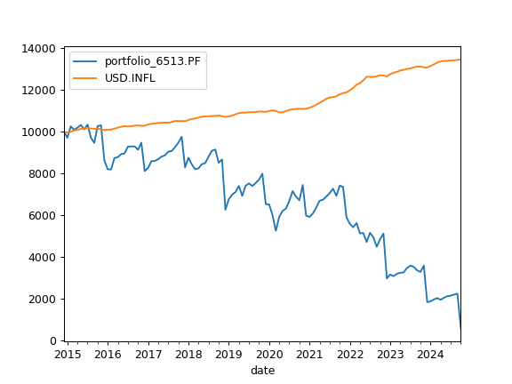
>>> pf = ok.Portfolio(first_date="2015-01", last_date="2024-10")  # create Portfolio with default parameters
>>> # Set Monte Carlo parameters
>>> pf.dcf.set_mc_parameters(distribution="lognorm", period=10, mc_number=100)
>>> # Set the cash flow strategy. It's required to generate random wealth indexes.
>>> ind = ok.IndexationStrategy(pf)  # create IndexationStrategy linked to the portfolio
>>> ind.initial_investment = 10_000  # add initial investments size
>>> ind.frequency = "year"  # set cash flow frequency
>>> ind.amount = -1_500  # set withdrawal size
>>> ind.indexation = "inflation"
>>> # Assign the strategy to Portfolio
>>> pf.dcf.cashflow_parameters = ind
>>> # Plot wealth index with cash flow
>>> pf.dcf.wealth_index(discounting="fv", include_negative_values=False).plot()
>>> plt.show()
- wealth_index(discounting, include_negative_values=False)
Calculate wealth index time series for the portfolio with cash flow (contributions and withdrawals) using historical rate of returns.
Wealth index (Cumulative Wealth Index) is a time series that presents the value of portfolio over historical time period considering cash flows.
Accumulated inflation time series is added if inflation=True in the Portfolio.
If there is no cash flow, Wealth index is obtained from the accumulated return multiplied by the initial investments. That is: initial_investment * (Accumulated_Return + 1)
- Parameters:
- discounting{‘fv’, ‘pv’}
Type of discounting to apply: - ‘fv’: Future Values - nominal values without discounting - ‘pv’: Present Values - values discounted to present using the discount rate
- include_negative_valuesbool, default False
Whether to include negative wealth index values in the result. If False, negative values are replaced with zeros.
- Returns:
- pd.DataFrame
Time series of wealth index values for portfolio and accumulated inflation (if applicable).
Examples
>>> import matplotlib.pyplot as plt
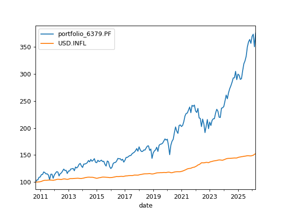
>>> pf = ok.Portfolio(["VOO.US", "GLD.US"], weights=[0.8, 0.2])
>>> ind = ok.IndexationStrategy(pf)  # Set Cash Flow Strategy parameters
>>> ind.initial_investment = 100  # initial investments value
>>> ind.frequency = "year"  # withdrawals frequency
>>> ind.amount = -6  # initial withdrawals amount
>>> ind.indexation = "inflation"  # the indexation is equal to inflation
>>> pf.dcf.cashflow_parameters = ind  # assign the strategy to Portfolio
>>> pf.dcf.wealth_index(discounting="fv", include_negative_values=False).plot()
>>> plt.show()
- cash_flow_ts(discounting, remove_if_wealth_index_negative=True)
Cash flow Future Values (FV) or Present Values (PV) time series for the portfolio.
The cash flow time series presents the values of contributions and withdrawals over historical time period.
- Parameters:
- discounting{‘fv’, ‘pv’}
Type of discounting to apply: - ‘fv’: Future Values - nominal values without discounting - ‘pv’: Present Values - values discounted to present using the discount rate
- remove_if_wealth_index_negativebool, default True
If True, cash flow values are replaced with 0 when wealth index is negative (or zero).
- Returns:
- pd.Series
Time series of cash flow values for portfolio.
Examples
>>> import matplotlib.pyplot as plt
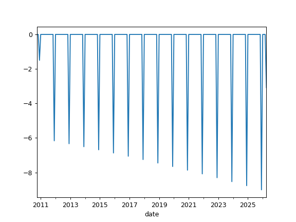
>>> pf = ok.Portfolio(["VOO.US", "GLD.US"], weights=[0.8, 0.2])
>>> ind = ok.IndexationStrategy(pf)  # Set Cash Flow Strategy parameters
>>> ind.initial_investment = 100  # initial investments value
>>> ind.frequency = "year"  # withdrawals frequency
>>> ind.amount = -0.5 * 12  # initial withdrawals amount
>>> ind.indexation = "inflation"  # the indexation is equal to inflation
>>> pf.dcf.cashflow_parameters = ind  # assign the strategy to Portfolio
>>> pf.dcf.cash_flow_ts(discounting="fv", remove_if_wealth_index_negative=True).plot()
>>> plt.show()
- irr()
Nominal internal rate of return (money-weighted return, MWRR) of the portfolio cash flow over the full historical period, honoring the configured cash flow strategy.
The cash-flow vector (investor perspective) on a monthly grid
t = 0 .. N, whereN = portfolio.ror.shape[0], is:t = 0(one month beforefirst_date):-initial_investmentt = 1 .. N:-cash_flow_ts(withdrawals become inflows, contributions outflows)t = N(last_date): additionally+the terminal wealth index value (liquidation; floored at 0, so the terminal withdrawal happens only if there is a positive balance left)
The annualized effective IRR is returned. With no intermediate cash flows the result equals
Portfolio.get_cagrfor the full period.IRR is a rate, so there is no future/present-value variant: discounting the flows would yield the real rate (the
get_cagr(real=True)axis), not “the IRR in PV”.- Returns:
- float
Annualized effective IRR. NaN if the cash flow has no sign change (no real root, e.g. pure accumulation with a zero terminal value). With contributions and withdrawals interleaved the equation may have several real roots; the root nearest the solver’s seed is returned.
Examples
>>> pf = ok.Portfolio(["SPY.US", "AGG.US"], ccy="USD", last_date="2024-10")
>>> ind = ok.IndexationStrategy(pf)
>>> ind.initial_investment = 10_000
>>> ind.frequency = "year"
>>> ind.amount = -1_000
>>> pf.dcf.cashflow_parameters = ind
>>> pf.dcf.irr()
- property wealth_index_fv_with_assets
Wealth index Future Values (FV) time series for the portfolio and all assets considering cash flow (contributions and withdrawals).
Wealth index (Cumulative Wealth Index) is a time series that presents the value of portfolio over historical time period. Accumulated inflation time series is added if inflation=True in the Portfolio.
If there is no cash flow, Wealth index is obtained from the accumulated return multiplied by the initial investments. That is: initial_investment * (Accumulated_Return + 1)
- Returns:
- DataFrame
Time series of wealth index values for portfolio, each asset and accumulated inflation.
Examples
>>> import matplotlib.pyplot as plt
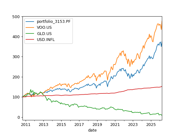
>>> pf = ok.Portfolio(["VOO.US", "GLD.US"], weights=[0.8, 0.2])
>>> ind = ok.IndexationStrategy(pf)  # Set Cash Flow Strategy parameters
>>> ind.initial_investment = 100  # initial investments value
>>> ind.frequency = "year"  # withdrawals frequency
>>> ind.amount = -0.5 * 12  # initial withdrawals amount
>>> ind.indexation = "inflation"  # the indexation is equal to inflation
>>> pf.dcf.cashflow_parameters = ind  # assign the strategy to Portfolio
>>> pf.dcf.wealth_index_fv_with_assets.plot()
>>> plt.show()
- survival_period_hist(threshold=0)
Calculate the period when the portfolio has positive balance considering withdrawals on the historical data.
The portfolio survival period (longevity period) depends on the investment strategy: asset allocation, rebalancing, withdrawals rate etc.
- Parameters:
- thresholdfloat, default 0
The percentage of the initial investments when the portfolio balance considered voided. This parameter is important to use in cash flow strategies with a fixed withdrawal percentage (PercentageStrategy).
- Returns:
- float
The portfolio survival period (longevity period) in years.
Examples
>>> pf = ok.Portfolio(["SPY.US", "AGG.US"], ccy="USD", first_date="2010-01", last_date="2024-10")
>>> # set cash flow strategy
>>> ind = ok.IndexationStrategy(pf)  # create cash flow strategy linked to the portfolio
>>> ind.initial_investment = 10_000  # add initial investment to cash flow strategy
>>> ind.amount = -2_500  # set annual withdrawal size
>>> ind.frequency = "year"  # set withdrawal frequency to year
>>> pf.dcf.cashflow_parameters = ind
>>> # Calculate the historical survival period for the cash flow strategy.
>>> # The balance is considered voided when it's equal to 0 (threshold=0)
>>> pf.dcf.survival_period_hist(threshold=0)
5.1
- survival_date_hist(threshold=0)
Get the date when the portfolio balance become negative considering withdrawals on the historical data.
The portfolio survival date (longevity date) depends on the investment strategy: asset allocation, rebalancing, withdrawals rate etc.
- Parameters:
- thresholdfloat, default 0
The percentage of the initial investments when the portfolio balance considered voided. This parameter is important to use in cash flow strategies with a fixed withdrawal percentage (PercentageStrategy).
- Returns:
- pd.Timestamp
The portfolio survival date.
Examples
>>> pf = ok.Portfolio(["SPY.US", "AGG.US"], ccy="USD", first_date="2010-01", last_date="2024-10")
>>> # set cash flow strategy
>>> ind = ok.IndexationStrategy(pf)  # create cash flow strategy linked to the portfolio
>>> ind.initial_investment = 10_000  # add initial investment to cash flow strategy
>>> ind.amount = -2_500  # set annual withdrawal size
>>> ind.frequency = "year"  # set withdrawal frequency to year
>>> pf.dcf.cashflow_parameters = ind
>>> # Calculate the historical survival period for the cash flow strategy
>>> pf.dcf.survival_date_hist(threshold=0)
Timestamp('2015-01-31 00:00:00')
- property initial_investment_pv
The discounted value (PV) of the initial investments at the historical first date.
- Returns:
- float or None
The discounted value (PV) of the initial investments at the historical first date.
Examples
>>> # Get discounted PV value of `initial_investment` for a portfolio with 4 years of history (at 2020-04).
>>> pf = ok.Portfolio(["EQMX.MOEX", "SBGB.MOEX"], ccy="RUB", last_date="2024-10")
>>> ind = ok.IndexationStrategy(pf)  # create cash flow strategy linked to the portfolio
>>> ind.initial_investment = 10_000  # add initial investment to cash flow strategy
>>> pf.dcf.cashflow_parameters = ind  # assign cash flow strategy to portfolio
>>> pf.dcf.discount_rate = 0.10  # define discount rate as 10%
>>> pf.dcf.initial_investment_pv
6574.643143611553
- property initial_investment_fv
The future value (FV) of the initial investments at the historical first date.
When the initial_investment parameter is not defined, initial_investment_fv is set to None.
- Returns:
- float or None
The future value (FV) of the initial investments.
Examples
>>> # Get discounted FV of initial_investment value for a period of 10 years.
>>> pf = ok.Portfolio(["EQMX.MOEX", "SBGB.MOEX"], ccy="RUB")
>>> ind = ok.IndexationStrategy(pf)  # create cash flow strategy linked to the portfolio
>>> ind.initial_investment = 10_000  # add initial investment to cash flow strategy
>>> pf.dcf.cashflow_parameters = ind  # assign cash flow strategy to portfolio
>>> pf.dcf.mc.period = 10  # define forecast period
>>> pf.dcf.discount_rate = 0.10  # define discount rate as 10%
>>> pf.dcf.initial_investment_fv
25937.424601000024
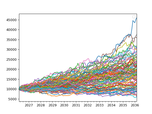
- monte_carlo_wealth(discounting='fv', include_negative_values=True)
Calculate portfolio random wealth indexes with cash flows (withdrawals/contributions) using Monte Carlo simulation.
Monte Carlo simulation generates n random monthly time series. Each wealth index is calculated with rate of return time series of a given distribution.
First date of forecasted returns is portfolio last_date. First value for the forecasted wealth indexes is the last historical portfolio index value. It is useful for a chart with historical wealth index and forecasted values.
- Parameters:
- discounting{‘fv’, ‘pv’}, default ‘fv’
‘fv’ - calculate Future Value (not discounted) wealth indexes. ‘pv’ - calculate Present Value (discounted) wealth indexes.
- include_negative_valuesbool, default True
If True, negative values in the wealth index are preserved. If False, negative values are replaced with 0.
- Returns:
- DataFrame
Table with n random wealth indexes monthly time series.
Examples
>>> import matplotlib.pyplot as plt
>>> pf = ok.Portfolio(
...     ["SPY.US", "AGG.US", "GLD.US"],
...     weights=[0.60, 0.35, 0.05],
...     rebalancing_strategy=ok.Rebalance(period="month"),
... )
>>> pf.dcf.set_mc_parameters(distribution="t", period=10, mc_number=100)  # Set Monte Carlo parameters
>>> # set cash flow parameters
>>> ind = ok.IndexationStrategy(pf)  # create cash flow strategy linked to the portfolio
>>> ind.initial_investment = 10_000  # add initial investment to cash flow strategy
>>> ind.amount = -500  # set withdrawal size
>>> ind.frequency = "year"  # set withdrawal frequency
>>> pf.dcf.cashflow_parameters = ind  # assign cash flow strategy to portfolio
>>> pf.dcf.monte_carlo_wealth(discounting="fv").plot()
>>> plt.legend("")  # don't show legend for each line
>>> plt.show()
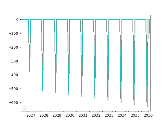
- monte_carlo_cash_flow(discounting, remove_if_wealth_index_negative=True)
Calculate portfolio random cash flow (withdrawals/contributions) time series by Monte Carlo simulation.
Monte Carlo simulation generates n random monthly time series of cash flows. Each cash flow time series corresponds to a wealth index calculated with rate of return time series of a given distribution.
First date of forecasted returns is portfolio last_date.
- Parameters:
- discounting{‘fv’, ‘pv’}
Type of discounting to apply: - ‘fv’: Future Values - nominal values without discounting - ‘pv’: Present Values - values discounted to present using the discount rate
- remove_if_wealth_index_negativebool, default True
If True, cash flow values are replaced with 0 when wealth index is negative (or zero).
- Returns:
- DataFrame
Table with n random cash flow monthly time series.
Examples
>>> import matplotlib.pyplot as plt
>>> pf = ok.Portfolio(
...     ["SPY.US", "AGG.US", "GLD.US"],
...     weights=[0.60, 0.35, 0.05],
...     rebalancing_strategy=ok.Rebalance(period="month"),
... )
>>> pf.dcf.set_mc_parameters(distribution="t", period=10, mc_number=100)  # Set Monte Carlo parameters
>>> # set cash flow parameters
>>> ind = ok.IndexationStrategy(pf)  # create cash flow strategy linked to the portfolio
>>> ind.initial_investment = 10_000  # add initial investment to cash flow strategy
>>> ind.amount = -500  # set withdrawal size
>>> ind.frequency = "year"  # set withdrawal frequency
>>> pf.dcf.cashflow_parameters = ind  # assign cash flow strategy to portfolio
>>> pf.dcf.monte_carlo_cash_flow(discounting="fv").plot()
>>> plt.legend("")  # don't show legend for each line
>>> plt.show()
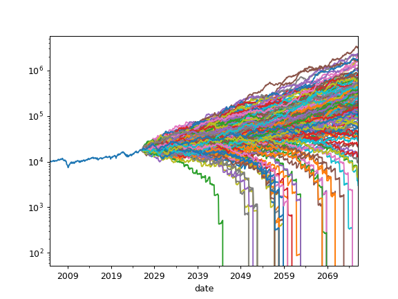
- plot_forecast_monte_carlo(backtest=True, figsize=None)
Plot Monte Carlo simulation for portfolio future wealth indexes optionally together with historical wealth index.
Wealth index (Cumulative Wealth Index) is a time series that presents the value of portfolio over time period considering cash flows (portfolio withdrawals/contributions).
Random wealth indexes are generated according to a given distribution.
- Parameters:
- backtestbool, default True
Include historical wealth index if True.
- figsizetuple of (float, float), default None
Figure size (width, height) in inches. If None, matplotlib defaults are used.
- Returns:
- Axes
Matplotlib axes object.
Examples
>>> import matplotlib.pyplot as plt
>>> pf = ok.Portfolio(
...     assets=["SPY.US", "AGG.US", "GLD.US"],
...     weights=[0.60, 0.35, 0.05],
...     rebalancing_strategy=ok.Rebalance(period="year"),
... )
>>> # Set Monte Carlo parameters
>>> pf.dcf.set_mc_parameters(distribution="norm", period=50, mc_number=200)
>>> # set cash flow parameters
>>> ind = ok.IndexationStrategy(pf)  # create cash flow strategy linked to the portfolio
>>> ind.initial_investment = 10_000  # add initial investment to cash flow strategy
>>> ind.amount = -500  # set withdrawal size
>>> ind.frequency = "year"  # set withdrawal frequency
>>> pf.dcf.cashflow_parameters = ind  # assign cash flow strategy to portfolio
>>> pf.dcf.plot_forecast_monte_carlo(backtest=True)
>>> plt.yscale("log")  # Y-axis has logarithmic scale
>>> plt.show()
- monte_carlo_survival_period(threshold=0)
Generate a survival period distribution for a portfolio with cash flows by Monte Carlo simulation.
Analyzing the result, finding “min”, “max” and percentiles it’s possible to see for how long will last the investment strategy - possible longevity period.
- Parameters:
- thresholdfloat, default 0
The percentage of the initial investments when the portfolio balance considered voided. This parameter is important to use in cash flow strategies with a fixed withdrawal percentage (PercentageStrategy).
- Returns:
- Series
Survival period distribution for a portfolio with cash flows.
Examples
>>> pf = ok.Portfolio(["SPY.US", "AGG.US", "GLD.US"], weights=[0.60, 0.35, 0.05])
>>> # set Monte Carlos parameters
>>> pf.dcf.set_mc_parameters(
...     distribution="t",  # use Student's distribution (t-distribution)
...     period=50,  # make forecast for 50 years
...     mc_number=200,  # create 200 randow wealth indexes
... )
>>> # Set Cash Flow parameters
>>> pc = ok.PercentageStrategy(pf)  # create PercentageStrategy linked to the portfolio
>>> pc.initial_investment = 10_000  # add initial investments size
>>> pc.frequency = "year"  # set cash flow frequency
>>> pc.percentage = -0.20  # set withdrawal percentage
>>> # Assign the strategy to Portfolio
>>> pf.dcf.cashflow_parameters = pc
>>> s = pf.dcf.monte_carlo_survival_period(threshold=0.10)  # the balance is considered voided at 10%
>>> s.min()
np.float64(10.5)
>>> s.max()
np.float64(33.5)
>>> s.mean()
np.float64(17.9055)
>>> s.quantile(50 / 100)
np.float64(17.5)
- monte_carlo_irr()
Distribution of money-weighted IRRs across Monte Carlo forecast paths.
For each simulated path the nominal internal rate of return (MWRR) is computed over the forecast horizon, honoring the configured cash flow strategy. It is the forward-looking counterpart of
irr().All paths share a single Monte Carlo return draw (see MonteCarlo.seed for reproducibility). The per-path investor cash-flow vector on a monthly grid
t = 0 .. M(M = mc.period * 12) is:t = 0(Monte Carlo start):-initial_investmentt = 1 .. M:-monte_carlo_cash_flow(withdrawals become inflows)t = M: additionally+the terminal wealth value (floored at 0)
With no intermediate cash flows each path’s IRR equals that path’s CAGR.
- Returns:
- Series
One annualized effective IRR per Monte Carlo path (length
mc_number). NaN for paths whose cash flow has no sign change.
Examples
>>> pf = ok.Portfolio(["SPY.US", "AGG.US"], ccy="USD")
>>> pf.dcf.set_mc_parameters(distribution="norm", period=20, mc_number=100, seed=0)
>>> ind = ok.IndexationStrategy(pf)
>>> ind.initial_investment = 10_000
>>> ind.frequency = "year"
>>> ind.amount = -500
>>> pf.dcf.cashflow_parameters = ind
>>> pf.dcf.monte_carlo_irr().quantile([0.1, 0.5, 0.9])
- find_the_largest_withdrawals_size(goal, withdrawals_range=(0, 1), target_survival_period=25, percentile=20, threshold=0, tolerance_rel=0.1, iter_max=20)
Find the largest withdrawal size for Monte Carlo simulation according to a cash flow strategy.
You can find the largest withdrawal size for three goals:
‘maintain_balance_pv’ to keep the purchasing power of the investments after inflation for the whole period defined in Monte Carlo parameters.
‘maintain_balance_fv’ to keep the nominal size of the investments for the whole period defined in Monte Carlo parameters.
‘survival_period’ to keep a positive balance for a period defined by target_survival_period.
The method works with IndexationStrategy, PercentageStrategy and their subclasses only.
The withdrawal size defined in cash flow strategy must be negative.
The result of finding a solution has the following parameters: - ‘success’ - whether the solution was found or not. - ‘withdrawal_abs’ - the absolute amount of withdrawal size (the best solution if found). - ‘withdrawal_rel’ - the relative amount of withdrawal size (the best solution if found). - ‘error_rel’ - characterizes how accurately the goal is fulfilled. - ‘solutions’ - the history of attempts to find solutions (withdrawal values and error level).
The algorithm evaluates the goal at both ends of withdrawals_range first and stops early if the solution lies outside the range; otherwise it finds the withdrawal size with Brent’s method (scipy.optimize.brentq) over the cached set of Monte Carlo scenarios.
- Parameters:
- goal{‘maintain_balance_fv’, ‘maintain_balance_pv’, ‘survival_period’}
‘maintain_balance_fv’ - the goal is to maintain the balance not lower than the nominal amount of the initial investment for the whole period defined in Monte Carlo parameters. ‘maintain_balance_pv’ - the goal is to keep the purchasing power of the investments after inflation for the whole period defined in Monte Carlo parameters. ‘survival_period’ - the goal is to keep positive balance for a period defined by ‘target_survival_period’.
- withdrawals_rangetuple of (float, float), default (0, 1)
The expected range of annualized withdrawal size measured as a percentage of the Initial Investment (CashFlow.initial_investment). 0.01 stands for 1%. (0.02, 0.05) means that expected withdrawal is in range from 2% to 5% of Initial Investment. The first value is expected minimum withdrawal. The second value is expected maximum withdrawal. The search for a solution occurs only within this range.
- percentileint, default 20
The percentile of Monte-Carlo simulation distribution where the goal is achieved. Percentile must be from 0 to 100. 1st or 5th percentiles are the examples of “bad” scenarios. 50th is median. 95th or 99th are optimistic scenarios.
- thresholdfloat, default 0
The percentage of initial investments when the portfolio balance is considered voided. Important for the “fixed_percentage” Cash flow strategy.
- target_survival_periodint, default 25
The smallest acceptable survival period. It works with the ‘survival_period’ goal only and is ignored for the ‘maintain_balance_pv’ and ‘maintain_balance_fv’ goals. For the ‘survival_period’ goal the value must be less than the MonteCarlo.period parameter.
- iter_maxint, default 20
The maximum number of objective evaluations (each runs one Monte Carlo simulation), including the two evaluations at the ends of withdrawals_range.
- tolerance_relfloat, default 0.10
The allowed tolerance for the solution. The tolerance is the largest error for the achieved goal.
- Returns:
- Result
The result of the solution search.
Examples
>>> pf = ok.Portfolio(
...     assets=["MCFTR.INDX", "RUCBTRNS.INDX"],
...     weights=[0.3, 0.7],
...     inflation=True,
...     ccy="RUB",
...     rebalancing_strategy=ok.Rebalance(period="year"),
... )
>>> # Fixed Percentage strategy
>>> pc = ok.PercentageStrategy(pf)
>>> pc.initial_investment = 10_000
>>> pc.frequency = "year"
>>> # Assign a strategy
>>> pf.dcf.cashflow_parameters = pc
>>> # Set Monte Carlo parameters (seed makes the search reproducible)
>>> pf.dcf.set_mc_parameters(distribution="norm", period=50, mc_number=200, seed=42)
>>> res = pf.dcf.find_the_largest_withdrawals_size(
...     percentile=50,
...     goal="survival_period",
...     threshold=0.05,
...     target_survival_period=25,
... )
>>> res
success                  True
withdrawal_abs   -1598.947236
withdrawal_rel       0.159895
error_rel               0.048
attempts                    7
dtype: object
In the result, withdrawal_abs is the absolute value of the withdrawal (the first withdrawal value), and withdrawal_rel is the relative withdrawal size (the first withdrawal value divided by the initial investment).
Even if the solution was not found, it is still possible to see the intermediate steps: the two evaluations at the range ends followed by the Brent root-finding steps. Exact values depend on the historical data window the distribution is fitted to.
>>> res.solutions
  withdrawal_abs withdrawal_rel error_rel error_rel_change
0       -10000.0              1     0.928                0
1            0.0              0       1.0            0.072
2   -5186.721992       0.518672     0.768           -0.232
3   -2593.360996       0.259336      0.46           -0.308
4   -1296.680498       0.129668     0.276           -0.184
5   -1782.935685       0.178294     0.168           -0.108
6   -1598.947236       0.159895     0.048            -0.12