![]()
You can run the code examples in Google Colab.
To install the package:
[5]:
%%capture --no-stderr
%pip install --quiet -U okama
Import okama and matplotlib packages.
[ ]:
import warnings

import matplotlib.pyplot as plt

import okama as ok

warnings.filterwarnings("ignore")

plt.rcParams["figure.figsize"] = [12.0, 6.0]
Get information about a single asset
You can start by getting general information about a single asset or index.
[7]:
one_asset = ok.Asset("VOO.US")
one_asset
[7]:
symbol                         VOO.US
name             Vanguard S&P 500 ETF
country                           USA
exchange                    NYSE ARCA
currency                          USD
type                              ETF
isin                     US9229083632
first date                    2010-10
last date                     2026-03
period length                   15.40
dtype: object
[8]:
# live (20 min delay) price
one_asset.price
[8]:
580.93
[9]:
# dividends history
one_asset.dividends.tail(10)
[9]:
date
2025-06    1.7447
2025-07    0.0000
2025-08    0.0000
2025-09    1.7400
2025-10    0.0000
2025-11    0.0000
2025-12    1.7710
2026-01    0.0000
2026-02    0.0000
2026-03    1.8724
Freq: M, Name: VOO.US, dtype: float64
Financial Database: Tickers & Namespaces
If you are unsure whether a ticker is available or how an asset is named, check it with search:
[10]:
ok.search("exxon")
[10]:
| symbol | ticker | name | country | exchange | currency | type | isin | |
|---|---|---|---|---|---|---|---|---|
| 0 | XOM.US | XOM | Exxon Mobil Corp | USA | NYSE | USD | Common Stock | US30231G1022 |
| 1 | XONA.XETR | XONA | Exxon Mobil Corporation | Germany | XETR | EUR | Common Stock | US30231G1022 |
| 2 | 0R1M.LSE | 0R1M | Exxon Mobil Corporation | UK | LSE | USD | Common Stock | US30231G1022 |
| 3 | XO3S.LSE | XO3S | Leverage Shares -3x Short Exxon (XOM) ETP Secu... | UK | LSE | USD | ETF | |
| 4 | XONA.XFRA | XONA | Exxon Mobil Corporation | Germany | XFRA | EUR | Common Stock | US30231G1022 |
| 5 | XONA.XSTU | XONA | EXXON MOBIL (XONA.SG) | Germany | XSTU | EUR | Common Stock | US30231G1022 |
A namespace is the set of characters after the period in a ticker (SPY.US).
Namespaces are based on MICs (Market Identifier Codes) and okama’s own codes for macroeconomic parameters.
[11]:
# available namespaces
ok.namespaces
[11]:
{'CBR': 'Central Banks official currency exchange rates',
 'CC': 'Cryptocurrency pairs with USD',
 'COMM': 'Commodities prices',
 'FX': 'FOREX currency market',
 'INDX': 'Indexes',
 'INFL': 'Inflation',
 'LSE': 'London Stock Exchange',
 'MOEX': 'Moscow Exchange',
 'PF': 'Investment Portfolios',
 'PIF': 'Russian open-end mutual funds',
 'RATE': 'Bank deposit rates',
 'RATIO': 'Financial ratios',
 'RE': 'Real estate prices',
 'US': 'US Stock Exchanges and mutual funds',
 'XAMS': 'Euronext Amsterdam',
 'XETR': 'XETRA Exchange',
 'XFRA': 'Frankfurt Stock Exchange',
 'XSTU': 'Stuttgart Exchange',
 'XTAE': 'Tel Aviv Stock Exchange (TASE)'}
[12]:
# available symbols in namespace
ok.symbols_in_namespace("INDX")
[12]:
| symbol | ticker | name | country | exchange | currency | type | isin | |
|---|---|---|---|---|---|---|---|---|
| 0 | 000906.INDX | 000906 | China Securities 800 | Unknown | INDX | CNY | INDEX | |
| 1 | 0O7N.INDX | 0O7N | Scale All Share GR EUR | Germany | INDX | EUR | INDEX | |
| 2 | 3LHE.INDX | 3LHE | ESTX 50 Corporate Bond TR | Greece | INDX | EUR | INDEX | |
| 3 | 5SP2550.INDX | 5SP2550 | S&P 500 Retailing (Industry Group) | USA | INDX | USD | INDEX | |
| 4 | 990100.INDX | 990100 | MSCI International World Index Price | Unknown | INDX | USD | INDEX | |
| ... | ... | ... | ... | ... | ... | ... | ... | ... |
| 2380 | XUSIN.INDX | XUSIN | BIST Industrials | Turkey | INDX | TRY | INDEX | |
| 2381 | XUSRD.INDX | XUSRD | BIST Sustainability | Turkey | INDEX | TRY | INDEX | |
| 2382 | XUTEK.INDX | XUTEK | BIST Technology | Turkey | INDEX | TRY | INDEX | |
| 2383 | YMU0.INDX | YMU0 | E-mini Dow $5 Future Sept 20 | USA | INDX | USD | Futures | |
| 2384 | YY1P.INDX | YY1P | EURO STOXX SMALL | USA | INDX | EUR | INDEX | CH0009107456 |
2385 rows × 8 columns
Compare assets from different stock markets
AssetList is used to compare different types of stocks, indexes, currencies, or commodities. Asset performance is adjusted to the base currency (USD by default).
[13]:
ls = ["SPY.US", "BND.US", "GC.COMM", "EUR.FX"]
currency = "EUR"  # base currency
[14]:
x = ok.AssetList(
    ls, ccy=currency, last_date="2020-01"
)  # first_date and last_date limits the Rate of Return time series
x
[14]:
assets           [SPY.US, BND.US, GC.COMM, EUR.FX]
currency                                       EUR
first_date                                 2007-05
last_date                                  2020-01
period_length                   12 years, 9 months
inflation                                 EUR.INFL
dtype: object
[15]:
x.names
[15]:
{'SPY.US': 'SPDR S&P 500 ETF Trust',
 'BND.US': 'Vanguard Total Bond Market Index Fund ETF Shares',
 'GC.COMM': 'Gold (COMEX)',
 'EUR.FX': 'US Dollar/Euro FX Cross Rate'}
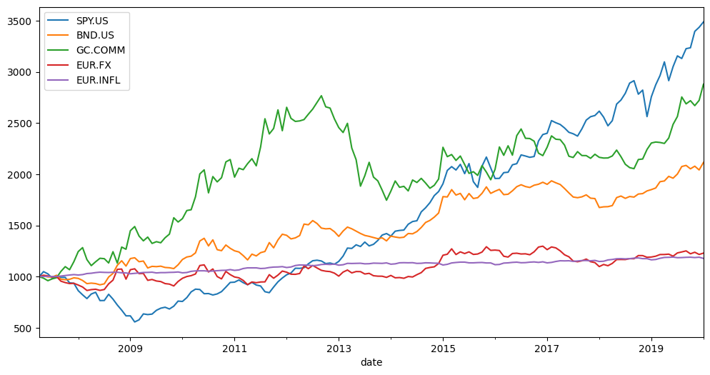
Let’s look at the accumulated return and compare it with inflation.
[16]:
x.wealth_indexes.plot();
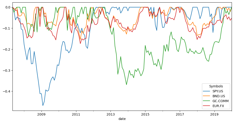
Drawdown history is also easy to inspect.
[17]:
x.drawdowns.plot();
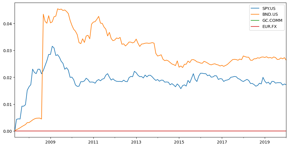
See the dividend yield history for all the assets in the list.
[18]:
x.dividend_yield.tail()
[18]:
| SPY.US | BND.US | GC.COMM | EUR.FX | |
|---|---|---|---|---|
| 2019-09 | 0.017978 | 0.026646 | 0.0 | 0.0 |
| 2019-10 | 0.017931 | 0.027154 | 0.0 | 0.0 |
| 2019-11 | 0.017083 | 0.026846 | 0.0 | 0.0 |
| 2019-12 | 0.017482 | 0.027272 | 0.0 | 0.0 |
| 2020-01 | 0.017219 | 0.026330 | 0.0 | 0.0 |
… or plot the same results.
[19]:
x.dividend_yield.plot();
The .describe() method shows the main parameters (risk metrics, rates of return, etc.) for the list of assets.
[20]:
x.describe(years=[1, 10]) # You can specify the period or leave the default: 1, 5 and 10 years
[20]:
| property | period | SPY.US | BND.US | GC.COMM | EUR.FX | inflation | |
|---|---|---|---|---|---|---|---|
| 0 | Compound return | YTD | 0.015294 | 0.035811 | 0.058055 | 0.0107 | -0.01 |
| 1 | CAGR | 1 years | 0.264954 | 0.143258 | 0.249053 | 0.031992 | 0.011915 |
| 2 | CAGR | 10 years | 0.164899 | 0.061206 | 0.062743 | 0.022543 | 0.012802 |
| 3 | CAGR | 12 years, 9 months | 0.102941 | 0.060522 | 0.086488 | 0.016364 | 0.01294 |
| 4 | Annualized mean return | 12 years, 9 months | 0.107585 | 0.063661 | 0.098019 | 0.021451 | NaN |
| 5 | Dividend yield | LTM | 0.017219 | 0.02633 | 0.0 | 0.0 | NaN |
| 6 | Risk | 12 years, 9 months | 0.150425 | 0.10467 | 0.19155 | 0.105235 | NaN |
| 7 | CVAR | 12 years, 9 months | 0.330952 | 0.128223 | 0.3078 | 0.155073 | NaN |
| 8 | Max drawdowns | 12 years, 9 months | -0.468342 | -0.153572 | -0.368852 | -0.173337 | NaN |
| 9 | Max drawdowns dates | 12 years, 9 months | 2009-02 | 2011-04 | 2013-12 | 2011-04 | NaN |
| 10 | Inception date | None | 1993-02 | 2007-05 | 1975-02 | 1975-02 | 1996-02 |
| 11 | Last asset date | None | 2020-01 | 2020-01 | 2020-01 | 2020-01 | 2020-01 |
| 12 | Common last data date | None | 2020-01 | 2020-01 | 2020-01 | 2020-01 | 2020-01 |
Correlation Matrix
If you need to check the correlation (or covariance) between asset returns, you can use native pandas functions.
Monthly rate-of-return time series are available through the .assets_ror property:
[21]:
x.assets_ror.tail()
[21]:
| Symbols | SPY.US | BND.US | GC.COMM | EUR.FX |
|---|---|---|---|---|
| date | ||||
| 2019-09 | 0.030714 | 0.005237 | -0.024587 | 0.0084 |
| 2019-10 | 0.002680 | -0.015959 | 0.011607 | -0.0227 |
| 2019-11 | 0.049567 | 0.012495 | -0.017791 | 0.0123 |
| 2019-12 | 0.011605 | -0.017688 | 0.019174 | -0.0174 |
| 2020-01 | 0.015294 | 0.035811 | 0.058055 | 0.0107 |
The correlation matrix can be obtained with x.assets_ror.corr().
[22]:
x.assets_ror.corr()
[22]:
| Symbols | SPY.US | BND.US | GC.COMM | EUR.FX |
|---|---|---|---|---|
| Symbols | ||||
| SPY.US | 1.000000 | 0.179704 | -0.085518 | 0.211607 |
| BND.US | 0.179704 | 1.000000 | 0.338168 | 0.907689 |
| GC.COMM | -0.085518 | 0.338168 | 1.000000 | 0.185743 |
| EUR.FX | 0.211607 | 0.907689 | 0.185743 | 1.000000 |
Covariance matrix:
[23]:
x.assets_ror.cov()
[23]:
| Symbols | SPY.US | BND.US | GC.COMM | EUR.FX |
|---|---|---|---|---|
| Symbols | ||||
| SPY.US | 0.001537 | 0.000200 | -0.000168 | 0.000246 |
| BND.US | 0.000200 | 0.000809 | 0.000483 | 0.000767 |
| GC.COMM | -0.000168 | 0.000483 | 0.002522 | 0.000277 |
| EUR.FX | 0.000246 | 0.000767 | 0.000277 | 0.000883 |
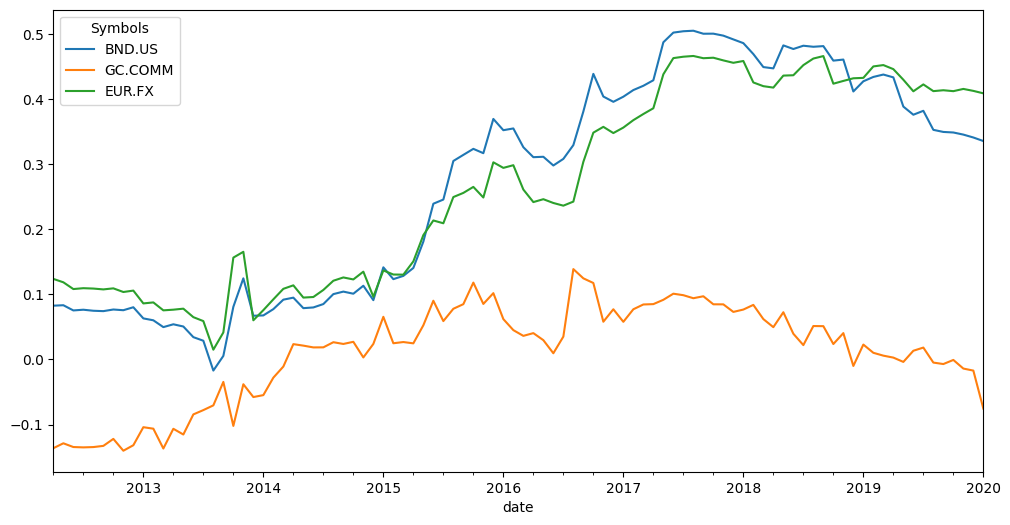
AssetList (SPY.US in this example).[24]:
x.index_corr(rolling_window=12 * 5).plot();
Basic portfolio methods
Let’s create a portfolio with three assets and USD as the base currency. We need to specify the weights.
[25]:
tickers = [
    "VNQ.US",
    "DBXD.XFRA",
    "MCFTR.INDX",
]  # we can create lists of assets and portfolio containing general type of assets and **indexes**
w = [0.5, 0.25, 0.25]
currency = "USD"
[26]:
y = ok.Portfolio(tickers, ccy=currency, weights=w)
y
[26]:
symbol                                     portfolio_2745.PF
assets                       [VNQ.US, DBXD.XFRA, MCFTR.INDX]
weights                                    [0.5, 0.25, 0.25]
rebalancing_period                                     month
rebalancing_abs_deviation                               None
rebalancing_rel_deviation                               None
currency                                                 USD
inflation                                           USD.INFL
first_date                                           2007-02
last_date                                            2026-02
period_length                             19 years, 1 months
dtype: object
[27]:
y.table
[27]:
| asset name | ticker | weights | |
|---|---|---|---|
| 0 | Vanguard Real Estate Index Fund ETF Shares | VNQ.US | 0.50 |
| 1 | Xtrackers - DAX UCITS ETF | DBXD.XFRA | 0.25 |
| 2 | MOEX Russia Total Return Index | MCFTR.INDX | 0.25 |
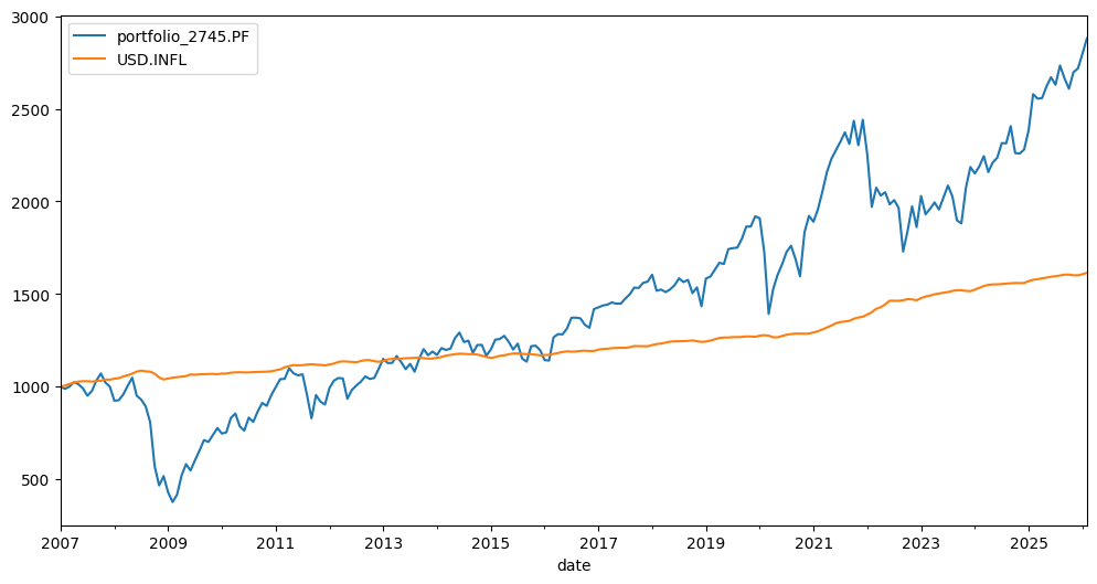
A portfolio has the same .wealth_index property (accumulated return) as an AssetList object.
[28]:
y.wealth_index.plot();
Risk metrics
You can use risk metrics such as volatility (standard deviation), semideviation, max drawdown, VaR, and CVaR.
[29]:
y.risk_annual.tail()
[29]:
date
2025-10    0.219978
2025-11    0.219891
2025-12    0.219411
2026-01    0.219229
2026-02    0.219067
Freq: M, Name: portfolio_2745.PF, dtype: float64
[30]:
y.semideviation_annual
[30]:
np.float64(0.17009760627025125)
[31]:
y.get_var_historic(level=1)
[31]:
np.float64(0.5422501601074122)
[32]:
y.get_cvar_historic(level=5)
[32]:
np.float64(0.46925923391795993)
[33]:
y.drawdowns.min()
[33]:
np.float64(-0.648114355818486)
.recovery_period.[34]:
y.recovery_period.max() / 12 # years
[34]:
np.float64(3.4166666666666665)
.describe() shows the main portfolio properties for different trailing periods.
[35]:
y.describe()
[35]:
| property | period | portfolio_2745.PF | inflation | |
|---|---|---|---|---|
| 0 | compound return | YTD | 0.059764 | 0.008417 |
| 1 | CAGR | 1 years | 0.116881 | 0.024041 |
| 2 | CAGR | 5 years | 0.080232 | 0.044380 |
| 3 | CAGR | 10 years | 0.097082 | 0.032603 |
| 4 | CAGR | 19 years, 1 months | 0.05701 | 0.025419 |
| 5 | Annualized mean return | 19 years, 1 months | 0.076655 | NaN |
| 6 | Dividend yield | LTM | 0.018141 | NaN |
| 7 | Risk | 19 years, 1 months | 0.219067 | NaN |
| 8 | CVAR (α=1) | 19 years, 1 months | 0.567506 | NaN |
| 9 | Max drawdown | 19 years, 1 months | -0.648114 | NaN |
| 10 | Max drawdown date | 19 years, 1 months | 2009-02 | NaN |