MonteCarlo
- class MonteCarlo(parent, distribution='norm', distribution_parameters=None, period=25, mc_number=100, seed=None)
Bases:
objectMonte Carlo simulation parameters for an investment portfolio.
- Parameters:
- parentPortfolioDCF
Parent PortfolioDCF instance.
- distribution{‘norm’, ‘lognorm’, ‘t’}, default ‘norm’
Distribution used to generate random monthly rates of return.
‘norm’ : Normal distribution.
‘lognorm’ : Lognormal distribution.
‘t’ : Student’s t-distribution.
- distribution_parameterstuple or None, default None
Parameters for the selected distribution. The expected tuple structure depends on distribution:
‘norm’ : (mu, sigma)
‘lognorm’ : (shape, loc, scale)
‘t’ : (df, loc, scale)
Any element can be None to indicate it should be inferred from the historical returns (for example, (3, None, None) fixes df=3 for the t-distribution and estimates loc and scale).
- periodint, default 25
Forecast horizon in years.
- mc_numberint, default 100
Number of random scenarios to generate.
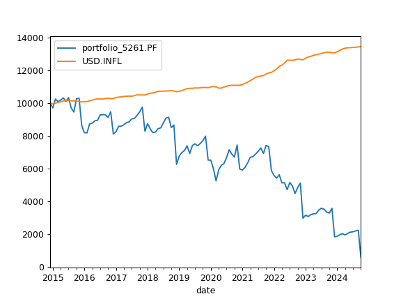
Examples
>>> import matplotlib.pyplot as plt
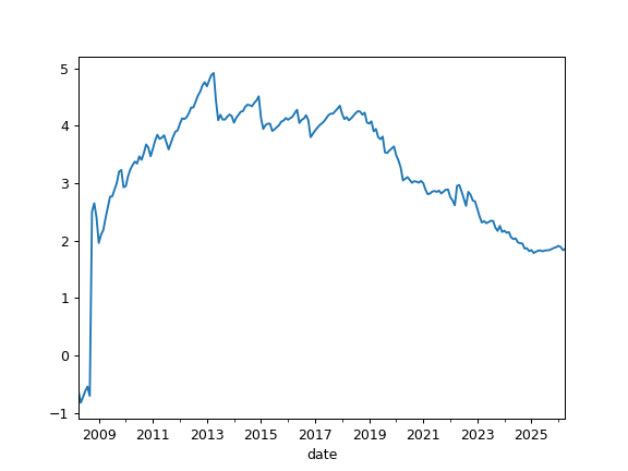
>>> pf = ok.Portfolio(first_date="2015-01", last_date="2024-10")
>>> pf.dcf.set_mc_parameters(distribution="t", period=10, mc_number=100)
>>> ind = ok.IndexationStrategy(pf)
>>> ind.initial_investment = 10_000
>>> ind.frequency = "year"
>>> ind.amount = -1_500
>>> ind.indexation = "inflation"
>>> pf.dcf.cashflow_parameters = ind
>>> pf.dcf.wealth_index(discounting="fv", include_negative_values=False).plot()
>>> plt.show()
Methods & Attributes
backtesting_error([var_level])Calculate Backtesting Error as the difference between empirical and theoretical risk measures (VaR, CVaR) and arithmetic mean.
Distribution used to generate random monthly rates of return.
Distribution parameters provided by the user for the selected distribution.
Resolve and return fully specified parameters for the current distribution.
Perform Jarque-Bera test for normality of portfolio returns time series.
Perform one sample Kolmogorov-Smirnov test on portfolio returns and evaluate goodness of fit for a given distribution.
Run Kolmogorov-Smirnov goodness-of-fit tests for all configured distributions.
Calculate expanding Fisher (normalized) kurtosis time series for portfolio rate of return.
kurtosis_rolling([window])Calculate rolling Fisher (normalized) kurtosis time series for portfolio rate of return.
Number of random scenarios to generate with Monte Carlo simulation.
Generate portfolio monthly rate of return time series with Monte Carlo simulation.
optimize_df_for_students(var_level)Find degrees of freedom for the t-distribution that best match empirical VaR and CVaR.
percentile_distribution_cagr([percentiles])Calculate percentiles for the simulated CAGR distribution.
percentile_inverse_cagr([score])Compute the percentile rank of a CAGR value within the simulated distribution.
Forecast period in years for portfolio wealth index time series.
plot_hist_fit([bins])Plot a histogram of historical monthly returns and overlay the fitted theoretical PDF.
plot_qq([var_level, bootstrap_size_var, ...])Generate a quantile-quantile (Q-Q) plot of portfolio monthly rate of return against quantiles of a given theoretical distribution.
Random seed for Monte Carlo return generation.
Compute expanding skewness time series for portfolio rate of return.
skewness_rolling([window])Compute rolling skewness of the return time series.
- property distribution
Distribution used to generate random monthly rates of return.
Allowed values:
‘norm’ : Normal distribution.
‘lognorm’ : Lognormal distribution.
‘t’ : Student’s t-distribution.
- Returns:
- str
- property distribution_parameters
Distribution parameters provided by the user for the selected distribution.
The expected tuple structure depends on the current distribution: - ‘norm’ : (mu, sigma) - ‘lognorm’ : (shape, loc, scale) - ‘t’ : (df, loc, scale)
Any element can be None to indicate it should be inferred from historical returns.
- Returns:
- tuple or None
Raw distribution parameters as configured. May contain None values.
- property period
Forecast period in years for portfolio wealth index time series.
- Returns:
- int
- property mc_number
Number of random scenarios to generate with Monte Carlo simulation.
- Returns:
- int
- property seed
Random seed for Monte Carlo return generation.
If None, each regeneration draws fresh randomness. Set an integer for reproducible scenarios. Changing the seed (or any other Monte Carlo parameter) invalidates the cached return draw.
- Returns:
- int or None
The configured random seed.
- backtesting_error(var_level=5)
Calculate Backtesting Error as the difference between empirical and theoretical risk measures (VaR, CVaR) and arithmetic mean.
- Parameters:
- var_levelint, default 5
Confidence level in percent for Value-at-Risk (VaR) and Conditional Value-at-Risk (CVaR). For example, 5 corresponds to 5% left tail.
- Returns:
- dict
Dictionary with the following keys:
- ‘delta_arithmetic_mean’: float
Difference between the theoretical and empirical arithmetic mean of returns.
- ‘delta_var’: float
Difference between empirical and theoretical Value-at-Risk at the specified level.
- ‘delta_cvar’: float
Difference between empirical and theoretical Conditional Value-at-Risk at the specified level.
- optimize_df_for_students(var_level)
Find degrees of freedom for the t-distribution that best match empirical VaR and CVaR.
The method minimizes the squared error between theoretical and empirical VaR/CVaR using scipy.optimize.minimize_scalar with bounds (2.1, 50).
- Parameters:
- var_levelint
Confidence level in percent for Value-at-Risk (VaR) and Conditional Value-at-Risk (CVaR). Must be in [1, 99].
- Returns:
- float
Estimated degrees of freedom for Student’s t-distribution.
- Raises:
- ValueError
If var_level is outside [1, 99].
- get_parameters_for_distribution()
Resolve and return fully specified parameters for the current distribution.
This method combines user-provided parameters (which may contain None values) with parameters estimated from the historical returns to produce a complete set of arguments for the selected distribution.
- Returns:
- tuple
A tuple of finalized parameters suitable for random variate generation and density/quantile calculations. The structure depends on the distribution:
‘norm’: (mu, sigma)
‘lognorm’: (shape, loc, scale) where loc is fixed at -1
‘t’: (df, loc, scale)
- Raises:
- ValueError
If the distribution is unknown.
- property monte_carlo_returns_ts
Generate portfolio monthly rate of return time series with Monte Carlo simulation.
Monte Carlo simulation generates n random monthly time series with a given distribution. Forecast period should not exceed 1/2 of portfolio history period length.
First date of forecaseted returns is portfolio last_date.
- Returns:
- DataFrame
Table with n random rate of return monthly time series.
Notes
The draw is generated once and cached: repeated accesses return the same scenarios until a Monte Carlo parameter changes (distribution, distribution_parameters, period, mc_number or seed), which invalidates the cache. Set seed for reproducible draws (see MonteCarlo.seed). This shared cache is what keeps monte_carlo_wealth and monte_carlo_cash_flow consistent on the same scenario set.
Examples
>>> pf = ok.Portfolio(
...     ["SPY.US", "AGG.US", "GLD.US"],
...     weights=[0.60, 0.35, 0.05],
...     rebalancing_strategy=ok.Rebalance(period="month"),
... )
>>> pf.dcf.set_mc_parameters(period=8, mc_number=5000, seed=0)
>>> pf.dcf.mc.monte_carlo_returns_ts
                 0         1         2     ...      4997      4998      4999
2021-07 -0.008383 -0.013167 -0.031659  ...  0.046717  0.065675  0.017933
2021-08  0.038773 -0.023627  0.039208  ... -0.016075  0.034439  0.001856
2021-09  0.005026 -0.007195 -0.003300  ... -0.041591  0.021173  0.114225
2021-10 -0.007257  0.003013 -0.004958  ...  0.037057 -0.009689 -0.003242
2021-11 -0.005006  0.007090  0.020741  ...  0.026509 -0.023554  0.010271
           ...       ...       ...  ...       ...       ...       ...
2029-02 -0.065898 -0.003673  0.001198  ...  0.039293  0.015963 -0.050704
2029-03  0.021215  0.008783 -0.017003  ...  0.035144  0.002169  0.015055
2029-04  0.002454 -0.016281  0.017004  ...  0.032535  0.027196 -0.029475
2029-05  0.011206  0.023396 -0.013757  ... -0.044717 -0.025613 -0.002066
2029-06 -0.016740 -0.007955  0.002862  ... -0.027956 -0.012339  0.048974
[96 rows x 5000 columns]
- percentile_distribution_cagr(percentiles=[10, 50, 90])
Calculate percentiles for the simulated CAGR distribution.
CAGR (Compound Annual Growth Rate) is calculated for each Monte Carlo return path.
- Parameters:
- percentileslist[int], default [10, 50, 90]
Percentiles to compute (0-100).
- Returns:
- dict[int, float]
Mapping {percentile: value}.
Examples
>>> pf = ok.Portfolio(
...     ["SPY.US", "AGG.US", "GLD.US"],
...     weights=[0.60, 0.35, 0.05],
...     rebalancing_strategy=ok.Rebalance(period="year"),
... )
>>> pf.dcf.set_mc_parameters(distribution="norm", period=1)
>>> pf.dcf.mc.percentile_distribution_cagr()
{10: ..., 50: ..., 90: ...}
>>> pf.dcf.set_mc_parameters(period=5)
>>> pf.dcf.mc.percentile_distribution_cagr([5, 10, 20])
{5: ..., 10: ..., 20: ...}
- percentile_inverse_cagr(score=0)
Compute the percentile rank of a CAGR value within the simulated distribution.
The percentile rank is calculated from the Monte Carlo CAGR distribution produced by the current Monte Carlo settings.
For example, if the percentile rank for score=0 is 8 for a 1-year horizon, it means that 8% of simulated CAGR values are negative over 1-year periods.
- Parameters:
- scorefloat, default 0
CAGR value to evaluate.
- Returns:
- float
Percentile rank (0-100).
Examples
>>> pf = ok.Portfolio(
...     ["SPY.US", "AGG.US", "GLD.US"],
...     weights=[0.60, 0.35, 0.05],
...     rebalancing_strategy=ok.Rebalance(period="year"),
... )
>>> pf.dcf.set_mc_parameters(distribution="lognorm", period=1, mc_number=5000)
>>> pf.dcf.mc.percentile_inverse_cagr(score=0)
...
The probability of getting negative result (score=0) in 1 year period for lognormal distribution.
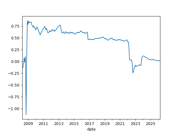
- property skewness
Compute expanding skewness time series for portfolio rate of return.
For normally distributed data, the skewness should be about zero. A skewness value greater than zero means that there is more weight in the right tail of the distribution.
- Returns:
- Series
Rolling skewness time series.
Examples
>>> pf = ok.Portfolio(["BND.US"])
>>> pf.dcf.mc.skewness
Date
2008-05   -0.134193
2008-06   -0.022349
2008-07    0.081412
2008-08   -0.020978
            ...
2021-04    0.441430
2021-05    0.445772
2021-06    0.437383
2021-07    0.425247
Freq: M, Name: portfolio_8378.PF, Length: 159, dtype: float64
>>> import matplotlib.pyplot as plt
>>> pf.dcf.mc.skewness.plot()
>>> plt.show()
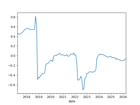
- skewness_rolling(window=60)
Compute rolling skewness of the return time series.
For normally distributed rate of return, the skewness should be about zero. A skewness value greater than zero means that there is more weight in the right tail of the distribution.
- Parameters:
- windowint, default 60
Size of the moving window in months. The window size should be at least 12 months.
- Returns:
- Series
Expanding skewness time series
Examples
>>> pf = ok.Portfolio(["BND.US"])
>>> pf.dcf.mc.skewness_rolling(window=12 * 10)
Date
2017-04    0.464916
2017-05    0.446095
2017-06    0.441211
2017-07    0.453947
2017-08    0.464805
...
2021-02    0.007622
2021-03    0.000775
2021-04    0.002308
2021-05    0.022543
2021-06   -0.006534
2021-07   -0.012192
Freq: M, Name: portfolio_8378.PF, dtype: float64
>>> import matplotlib.pyplot as plt
>>> pf.dcf.mc.skewness_rolling(window=12 * 10).plot()
>>> plt.show()
- property kurtosis
Calculate expanding Fisher (normalized) kurtosis time series for portfolio rate of return.
Kurtosis is a measure of whether the rate of return are heavy-tailed or light-tailed relative to a normal distribution. It should be close to zero for normally distributed rate of return. Kurtosis is the fourth central moment divided by the square of the variance.
- Returns:
- Series
Expanding kurtosis time series
Examples
>>> pf = ok.Portfolio(["BND.US"])
>>> pf.dcf.mc.kurtosis
Date
2008-05   -0.815206
2008-06   -0.718330
2008-07   -0.610741
2008-08   -0.534105
            ...
2021-04    2.821322
2021-05    2.855267
2021-06    2.864717
2021-07    2.850407
Freq: M, Name: portfolio_4411.PF, Length: 159, dtype: float64
>>> import matplotlib.pyplot as plt
>>> pf.dcf.mc.kurtosis.plot()
>>> plt.show()
- kurtosis_rolling(window=60)
Calculate rolling Fisher (normalized) kurtosis time series for portfolio rate of return.
Kurtosis is a measure of whether the rate of return are heavy-tailed or light-tailed relative to a normal distribution. It should be close to zero for normally distributed rate of return. Kurtosis is the fourth central moment divided by the square of the variance.
- Parameters:
- windowint, default 60
Size of the moving window in months. The window size should be at least 12 months.
- Returns:
- Series
Rolling kurtosis time series.
Examples
>>> pf = ok.Portfolio(["BND.US"])
>>> pf.dcf.mc.kurtosis_rolling(window=12 * 10)
Date
2017-04    4.041599
2017-05    4.133518
2017-06    4.165099
2017-07    4.205125
2017-08    4.313773
...
2021-03    0.362184
2021-04    0.409680
2021-05    0.455760
2021-06    0.457315
2021-07    0.496168
Freq: M, Name: portfolio_4411.PF, dtype: float64
>>> import matplotlib.pyplot as plt
>>> pf.dcf.mc.kurtosis_rolling(window=12 * 10).plot()
>>> plt.show()
- property jarque_bera
Perform Jarque-Bera test for normality of portfolio returns time series.
Jarque-Bera shows whether the returns have the skewness and kurtosis matching a normal distribution (null hypothesis or H0).
- Returns:
- dict
Jarque-Bera test statistics and p-value.
Notes
Test returns statistics (first row) and p-value (second row). p-value is the probability of obtaining test results, under the assumption that the null hypothesis is correct. In general, a large Jarque-Bera statistics and tiny p-value indicate that null hypothesis is rejected and the time series are not normally distributed.
Examples
>>> pf = ok.Portfolio(["BND.US"])
>>> pf.dcf.mc.jarque_bera
{'statistic': 58.27670538027455, 'p-value': 2.2148949341271873e-13}
- property kstest
Perform one sample Kolmogorov-Smirnov test on portfolio returns and evaluate goodness of fit for a given distribution.
The one-sample Kolmogorov-Smirnov test compares the rate of return time series against a given distribution.
- Returns:
- dict
Kolmogorov-Smirnov test statistics and p-value.
Notes
Like in Jarque-Bera test returns statistic (first row) and p-value (second row). Null hypotesis (two distributions are similar) is not rejected when p-value is high enough. 5% threshold can be used.
Examples
>>> pf = ok.Portfolio(["GLD.US"])
>>> pf.dcf.set_mc_parameters(distribution="lognorm")
>>> pf.dcf.mc.kstest
{'statistic': 0.05001344986084533, 'p-value': 0.6799422889377373}
>>> pf.dcf.set_mc_parameters(distribution="norm")
>>> pf.dcf.mc.kstest
{'statistic': 0.09528000069992831, 'p-value': 0.047761781235967415}
Kolmogorov-Smirnov test shows that GLD rate of return time series fits lognormal distribution better than normal one.
- property kstest_for_all_distributions
Run Kolmogorov-Smirnov goodness-of-fit tests for all configured distributions.
This property evaluates the KS test of the instance’s return series against each distribution defined in the project’s configured list of distributions and aggregates the results into a single DataFrame.
- Returns:
- pandas.DataFrame
A DataFrame where the index contains distribution names and each row holds the KS test results for that distribution (e.g., test statistic and p-value). The exact column labels depend on the underlying test implementation.
See also
kstestRun the KS test for a single distribution.
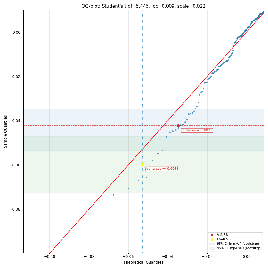
- plot_qq(var_level=5, bootstrap_size_var=2000, zoom_to_left_tail=20, figsize=None)
Generate a quantile-quantile (Q-Q) plot of portfolio monthly rate of return against quantiles of a given theoretical distribution.
A q-q plot is a plot of the quantiles of the portfolio rate of return historical data against the quantiles of a given theoretical distribution.
Bootstrap bands in a Q–Q plot are bootstrap-based confidence envelopes around quantiles that show the amount of random sample-to-sample variation one would expect. They bands built by repeatedly resampling dataset of a given size and recomputing the Q–Q points.
- Parameters:
- var_levelint, default 5
Confidence level in percent for VaR and CVaR.
- bootstrap_size_varint, default 2000
Number of bootstrap resamples used to compute confidence intervals for empirical VaR and CVaR. If 0, the bootstrap stripe is not drawn. A larger number provides a smoother estimate of the confidence bands at the cost of computation time.
- zoom_to_left_tailint or None, default 20
Zoom the plot to the left tail by limiting the view to the [0.1%, zoom_to_left_tail`%] percentile range. Must be in [1, 98]. Use `None to show the full range.
- figsizetuple[float, float], default None
Figure size in inches (width, height). If None, matplotlib default is used.
- Returns:
- Axes
Matplotlib axes object.
Examples
>>> import matplotlib.pyplot as plt
>>> pf = ok.Portfolio(
...     ["SPY.US", "AGG.US", "GLD.US"],
...     weights=[0.60, 0.35, 0.05],
...     rebalancing_strategy=ok.Rebalance(period="year"),
... )
>>> pf.dcf.set_mc_parameters(distribution="t")
>>> pf.dcf.mc.plot_qq(bootstrap_size_var=2000, zoom_to_left_tail=50, figsize=(10, 10))
>>> plt.show()
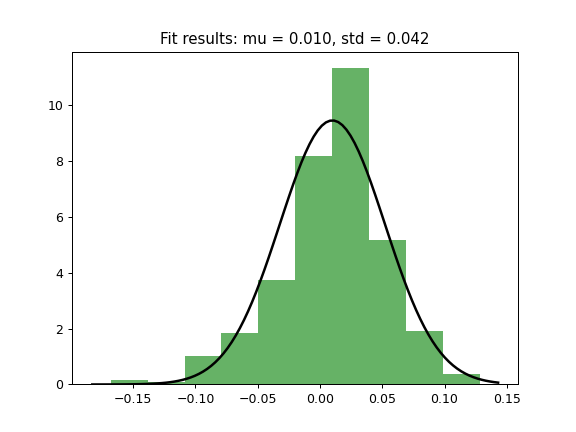
- plot_hist_fit(bins=None)
Plot a histogram of historical monthly returns and overlay the fitted theoretical PDF.
Uses the currently selected distribution (self.distribution) and its resolved parameters to draw the probability density function.
- Parameters:
- binsint, default None
Number of histogram bins. If None, matplotlib will choose automatically.
- Returns:
- Axes
Matplotlib axes object.
Examples
>>> import matplotlib.pyplot as plt
>>> pf = ok.Portfolio(["SP500TR.INDX"])
>>> pf.dcf.set_mc_parameters(distribution="norm")
>>> pf.dcf.mc.plot_hist_fit()
>>> plt.show()