plot_pair_ef

EfficientFrontier.plot_pair_ef(tickers='tickers', figsize=None)

Plot Efficient Frontier for every pair of assets.

Efficient Frontier is a set of portfolios which satisfy the condition that no other portfolio exists with a higher expected return but with the same risk (standard deviation of return).

Parameters:

tickers{‘tickers’, ‘names’} or list[str], default ‘tickers’

Annotation type for assets. ‘tickers’ - assets symbols are shown in form of ‘SPY.US’ ‘names’ - assets names are used like - ‘SPDR S&P 500 ETF Trust’ To show custom annotations for each asset pass the list of names.

figsizetuple[float, float], default None

Figure size (width, height) in inches. If None, matplotlib default is used.

Returns:

Axes

Matplotlib axes with the plot.

Notes

At least 3 assets are required.

Examples

>>> import matplotlib.pyplot as plt

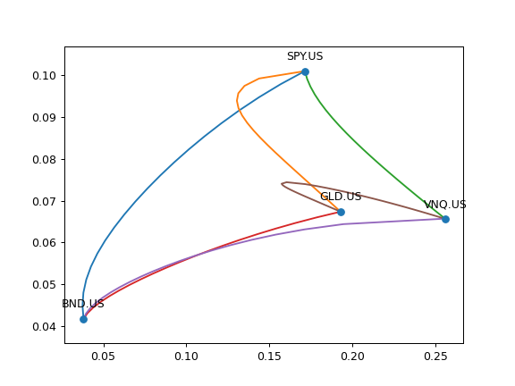
>>> ls4 = ["SPY.US", "BND.US", "GLD.US", "VNQ.US"]
>>> curr = "USD"
>>> last_date = "2021-07"
>>> ef = ok.EfficientFrontier(ls4, ccy=curr, last_date=last_date)
>>> ef.plot_pair_ef()
>>> plt.show()

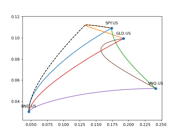
It can be useful to plot the full Efficient Frontier (EF) with optimized 4 asset portfolios together with the EFs for each pair of assets.

>>> ef4 = ok.EfficientFrontier(assets=ls4, ccy=curr, n_points=100)
>>> df4 = ef4.ef_points
>>> fig = plt.figure()
>>> # Plot Efficient Frontier for every pair of assets. Optimized portfolios will have 2 assets.
>>> ef4.plot_pair_ef()  # CAGR is used for optimized portfolios.
>>> ax = plt.gca()
>>> # Plot the full Efficient Frontier for 4 asset portfolios.
>>> ax.plot(df4["Risk"], df4["CAGR"], color="black", linestyle="--")
>>> plt.show()