plot_qq

MonteCarlo.plot_qq(var_level=5, bootstrap_size_var=2000, zoom_to_left_tail=20, figsize=None)

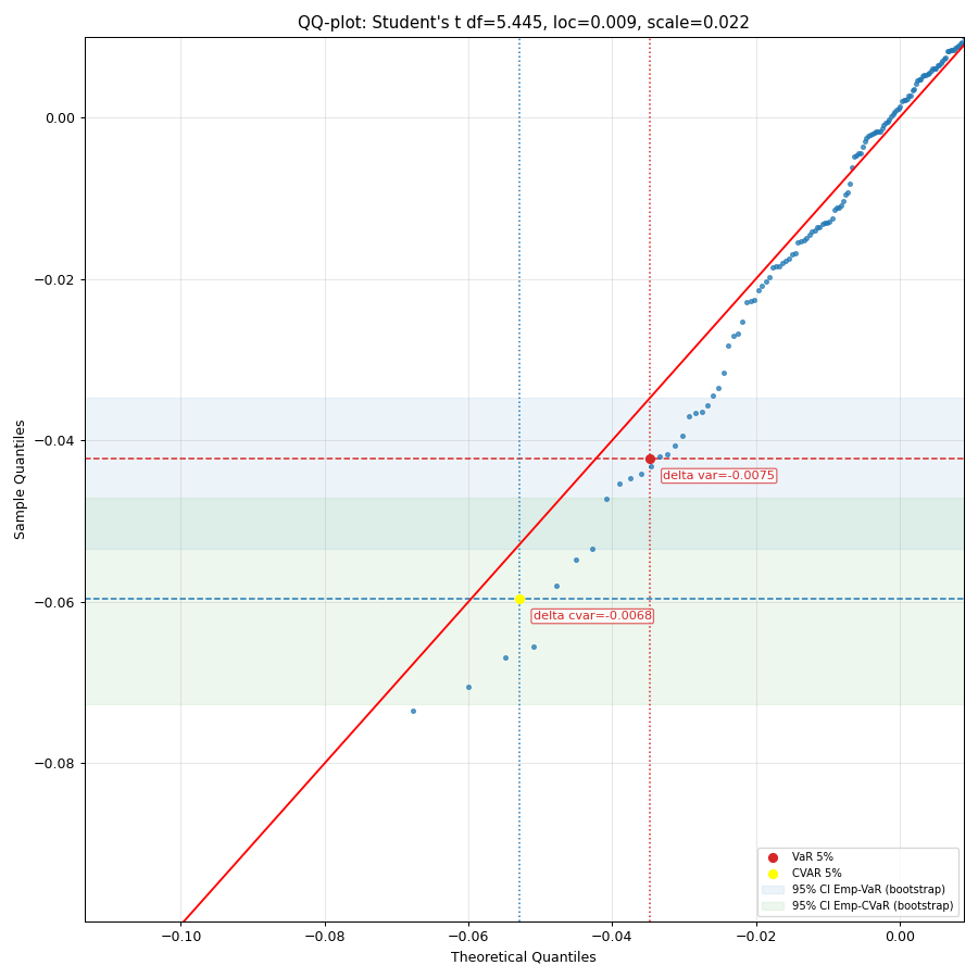
Generate a quantile-quantile (Q-Q) plot of portfolio monthly rate of return against quantiles of a given theoretical distribution.

A q-q plot is a plot of the quantiles of the portfolio rate of return historical data against the quantiles of a given theoretical distribution.

Bootstrap bands in a Q–Q plot are bootstrap-based confidence envelopes around quantiles that show the amount of random sample-to-sample variation one would expect. They bands built by repeatedly resampling dataset of a given size and recomputing the Q–Q points.

Parameters:

var_levelint, default 5

Confidence level in percent for VaR and CVaR.

bootstrap_size_varint, default 2000

Number of bootstrap resamples used to compute confidence intervals for empirical VaR and CVaR. If 0, the bootstrap stripe is not drawn. A larger number provides a smoother estimate of the confidence bands at the cost of computation time.

zoom_to_left_tailint or None, default 20

Zoom the plot to the left tail by limiting the view to the [0.1%, zoom_to_left_tail`%] percentile range. Must be in [1, 98]. Use `None to show the full range.

figsizetuple[float, float], default None

Figure size in inches (width, height). If None, matplotlib default is used.

Returns:

Axes

Matplotlib axes object.

Examples

>>> import matplotlib.pyplot as plt

>>> pf = ok.Portfolio(
...     ["SPY.US", "AGG.US", "GLD.US"],
...     weights=[0.60, 0.35, 0.05],
...     rebalancing_strategy=ok.Rebalance(period="year"),
... )
>>> pf.dcf.set_mc_parameters(distribution="t")
>>> pf.dcf.mc.plot_qq(bootstrap_size_var=2000, zoom_to_left_tail=50, figsize=(10, 10))
>>> plt.show()