![]()
You can run the code examples in Google Colab.
To install the package:
[ ]:
%%capture --no-stderr
%pip install --quiet -U okama
import okama and matplotlib packages …
[1]:
import warnings

import matplotlib.pyplot as plt

import okama as ok

warnings.simplefilter(action="ignore", category=FutureWarning)

plt.rcParams["figure.figsize"] = [12.0, 6.0]
Portfolio and AssetList are helpful for studying portfolio properties and comparing portfolios with each other. With AssetList, we can even compare a portfolio with stocks, indexes, and other financial assets, because a portfolio is just a special case of a financial asset.
In this tutorial we will learn how to:
create an investment portfolio and inspect its basic properties
understand rebalancing strategies and asset allocation
measure portfolio risk
analyze accumulated return, CAGR, and dividend yield
compare several portfolios
forecast portfolio performance
Create an investment portfolio
Portfolios are quite similar to AssetList, but we need to specify weights and a rebalancing strategy.
All arguments have default values and can be omitted.
[2]:
basic_portfolio = ok.Portfolio()
basic_portfolio
[2]:
symbol                        portfolio_4992.PF
assets                                 [SPY.US]
weights                                   [1.0]
rebalancing_period                        month
rebalancing_abs_deviation                  None
rebalancing_rel_deviation                  None
currency                                    USD
inflation                              USD.INFL
first_date                              1993-02
last_date                               2025-09
period_length                32 years, 8 months
dtype: object
SPY.US.USD.inflation=True.Rebalancing is the process by which an investor restores a portfolio to its target allocation by selling and buying assets. After rebalancing, all assets return to their original weights.
In the rebalancing strategy, the period can be: month, year, half-year, quarter, or none (for portfolios without rebalancing).
[3]:
rf3 = ok.Portfolio(
    ["BND.US", "VTI.US", "VXUS.US"],
    weights=[0.40, 0.40, 0.20],
    rebalancing_strategy=ok.Rebalance(period="year"),  # set the rebalancing period
)
rf3
[3]:
symbol                               portfolio_9868.PF
assets                       [BND.US, VTI.US, VXUS.US]
weights                                [0.4, 0.4, 0.2]
rebalancing_period                                year
rebalancing_abs_deviation                         None
rebalancing_rel_deviation                         None
currency                                           USD
inflation                                     USD.INFL
first_date                                     2011-02
last_date                                      2025-09
period_length                       14 years, 8 months
dtype: object
.assets_first_dates and .assets_last_dates.[4]:
rf3.assets_first_dates
[4]:
{'USD': Timestamp('1913-02-01 00:00:00'),
 'VTI.US': Timestamp('2001-06-01 00:00:00'),
 'BND.US': Timestamp('2007-05-01 00:00:00'),
 'VXUS.US': Timestamp('2011-02-01 00:00:00'),
 'USD.INFL': Timestamp('1913-02-01 00:00:00')}
[5]:
rf3.newest_asset
[5]:
'VXUS.US'
Here, VXUS.US is the asset with the shortest history, so it limits the history available for the entire portfolio.
[6]:
rf3.assets_last_dates
[6]:
{'BND.US': Timestamp('2025-11-01 00:00:00'),
 'VTI.US': Timestamp('2025-11-01 00:00:00'),
 'VXUS.US': Timestamp('2025-11-01 00:00:00'),
 'USD': Timestamp('2099-12-01 00:00:00'),
 'USD.INFL': Timestamp('2025-09-01 00:00:00')}
Inflation can also limit the available history. If you want to include the latest month even when inflation data is not yet available, instantiate the portfolio with inflation=False.
symbol= when creating the portfolio or set it afterward:[7]:
rf3.symbol = "RF3_portfolio.PF" # 'PF' namespace is reserved for portfolios.
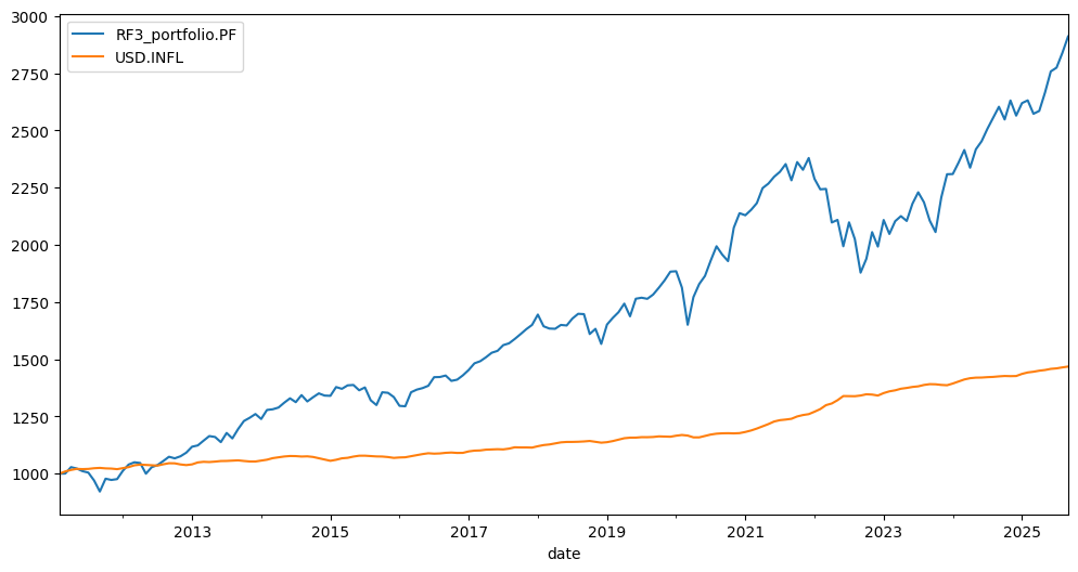
The wealth index (Cumulative Wealth Index) is a time series that shows the portfolio value over the historical period. The initial investment is 1,000 units of the base currency.
[8]:
rf3.wealth_index.plot();
Rebalancing strategy and asset allocation
The original asset-allocation table is available through .table:
[9]:
rf3.table
[9]:
| asset name | ticker | weights | |
|---|---|---|---|
| 0 | Vanguard Total Bond Market Index Fund ETF Shares | BND.US | 0.4 |
| 1 | Vanguard Total Stock Market Index Fund ETF Shares | VTI.US | 0.4 |
| 2 | Vanguard Total International Stock Index Fund ... | VXUS.US | 0.2 |
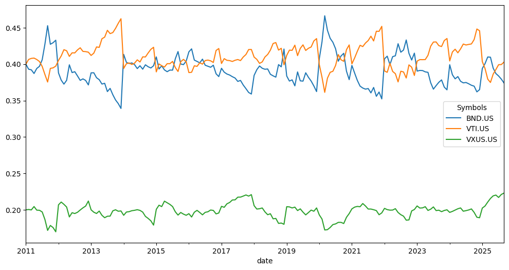
.weights_ts:[10]:
rf3.weights_ts.plot();
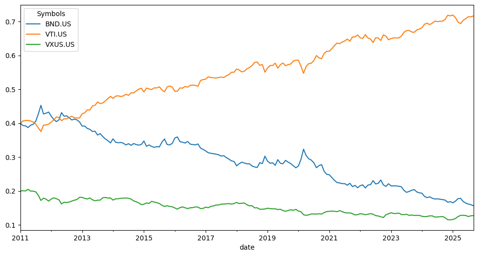
Let’s create the same Rick Ferri portfolio, but without rebalancing. In that case, the asset allocation will drift and never return to the original weights.
[11]:
rf3_no_rebalancing = ok.Portfolio(
    ["BND.US", "VTI.US", "VXUS.US"],
    weights=[0.40, 0.40, 0.20],
    rebalancing_strategy=ok.Rebalance(period="none"),
)
Now it is easy to see how the weights drift over time, and the portfolio ends up overweight in stocks.
[12]:
rf3_no_rebalancing.weights_ts.plot();
Risk metrics of the portfolio
A portfolio has several methods for inspecting risk metrics. By default, risk means the standard deviation of the return time series:
risk_monthly(standard deviation of monthly returns)risk_annual(annualized standard deviation)semideviation_monthly(downside risk for monthly returns)semideviation_annual(annualized semideviation)get_var_historic(historical Value at Risk for the portfolio)get_cvar_historic(historical Conditional Value at Risk for the portfolio)drawdowns(percentage decline from a previous peak)recovery_period(the longest recovery period after a drawdown in portfolio value)
[13]:
rf3.risk_annual.tail() # aanualized values time series for standard deviation of return
[13]:
date
2025-05    0.100104
2025-06    0.100318
2025-07    0.100023
2025-08    0.099949
2025-09    0.099924
Freq: M, Name: RF3_portfolio.PF, dtype: float64
[14]:
rf3.semideviation_annual # annualized value for downside risk
[14]:
np.float64(0.07586435955895295)
[15]:
rf3.get_cvar_historic(time_frame=12, level=1) # one year CVAR with confidence level 1%
[15]:
np.float64(0.1779330903217476)
Drawdowns (the percent decline from a previous peak) are easy to plot …
[16]:
rf3.drawdowns.plot();
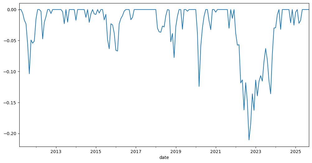
[17]:
rf3.drawdowns.nsmallest(5) # 5 Biggest drawdowns
[17]:
date
2022-09   -0.210563
2022-10   -0.185137
2022-12   -0.162683
2022-06   -0.162101
2022-08   -0.148924
Freq: M, Name: RF3_portfolio.PF, dtype: float64
recovery_period is closely related to drawdowns. It shows the longest recovery period for the portfolio value after a drawdown.
[18]:
rf3.recovery_period.nlargest() / 12 # we want it in years
[18]:
date
2024-02    2.166667
2016-06    1.083333
2012-01    0.750000
2018-07    0.500000
2019-02    0.500000
Freq: M, Name: RF3_portfolio.PF, dtype: float64
Accumulated return, CAGR and dividend yield
A portfolio has several metrics that can be used to measure returns and income:
wealth_index(the value of the portfolio over the historical period)wealth_index_with_assets(wealth index together with underlying asset values)mean_return_monthly(arithmetic mean of the portfolio return)mean_return_annual(annualized value of the monthly mean)annual_return_ts(calendar-year return time series)get_cagr(Compound Annual Growth Rate for a given trailing period)get_rolling_cagr(rolling CAGR)get_cumulative_return(expanding cumulative return time series over a given trailing period)get_rolling_cumulative_return(rolling cumulative return)dividend_yield(portfolio LTM dividend-yield monthly time series)
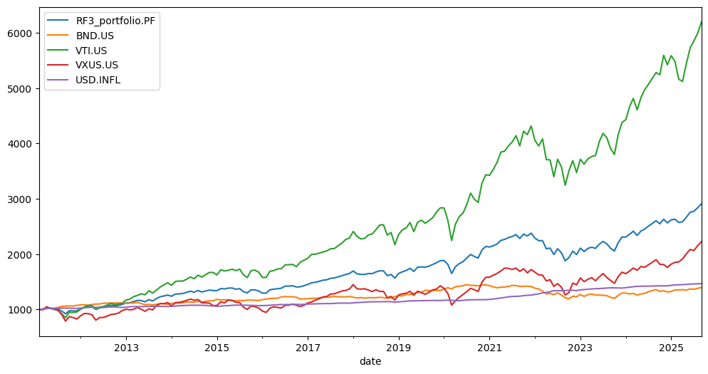
The wealth index is the simplest time series for showing portfolio value growth (we have already seen it above). Sometimes it is useful to compare portfolio growth with the growth of the underlying assets. For that, use wealth_index_with_assets.
[19]:
rf3.wealth_index_with_assets.plot();
The mean portfolio return can be annualized from the monthly mean:
[20]:
rf3.mean_return_annual
[20]:
np.float64(0.07778090663476697)
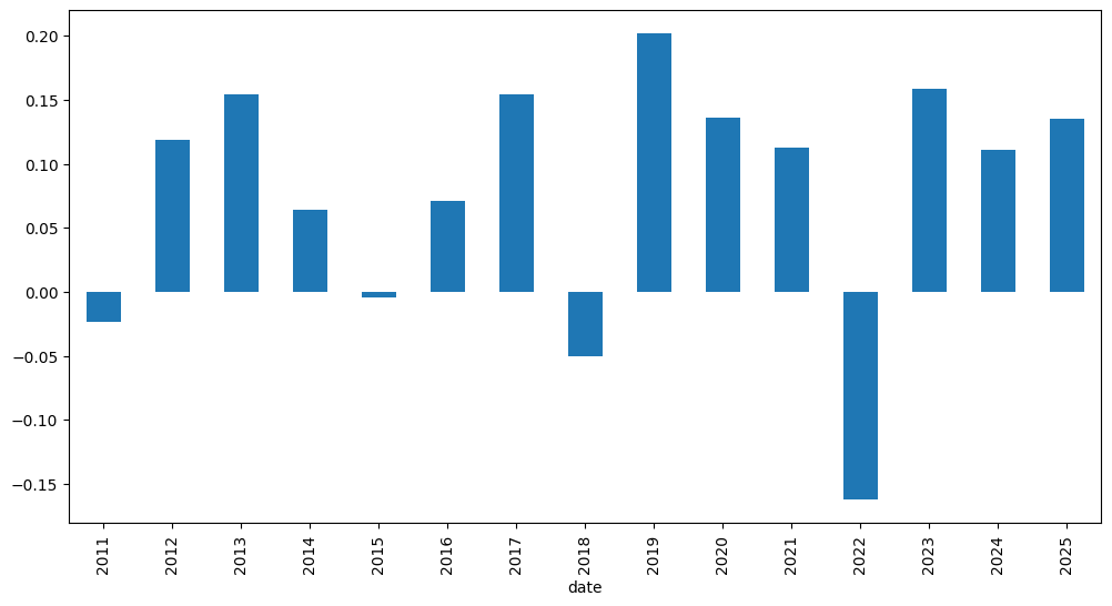
It is always useful to see how the portfolio performed on a calendar-year basis. The annual return time series shows the portfolio return for each year:
[24]:
rf3.annual_return_ts(return_type="cagr").tail() # can be cagr or arithmetic_mean
[24]:
date
2021    0.112746
2022   -0.162683
2023    0.158682
2024    0.110973
2025    0.134785
Freq: Y-DEC, Name: RF3_portfolio.PF, dtype: float64
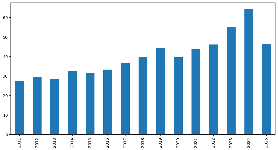
… or as a bar chart:
[26]:
rf3.annual_return_ts(return_type="cagr").plot(kind="bar");
One of the most important return metrics is CAGR (Compound Annual Growth Rate). It can be seen for trailing periods (parameter period is in years):
[27]:
rf3.get_cagr(period=5) # portfolio is initiated with inflation=True. Hence, we see CAGR with mean inflation.
[27]:
RF3_portfolio.PF    0.082588
USD.INFL            0.045298
dtype: float64
[28]:
rf3.get_cagr(period=5, real=True) # when real=True CAGR is adjusted for inflation (real CAGR)
[28]:
RF3_portfolio.PF    0.035674
dtype: float64
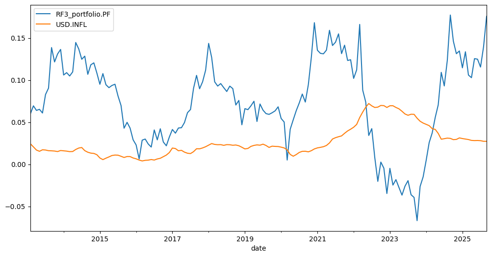
Rolling CAGR for the portfolio is available with get_rolling_cagr:
[29]:
rf3.get_rolling_cagr(
    window=12 * 2
).plot();  # window size is in months. We have rolling 2 year CAGR here and rolling 2 year mean inflation ...
The expanding cumulative return time series over a given trailing period can be calculated with get_cumulative_return. The period argument can be expressed in years or as YTD (Year to Date). The last row of the returned DataFrame is the cumulative return over the full selected period.
[ ]:
rf3.get_cumulative_return(
    period="YTD"
).tail()  # Cumulative return time series since the start of the current calendar year
[ ]:
rf3.get_cumulative_return(period=5).plot(); # Expanding cumulative return time series over the 5 years period
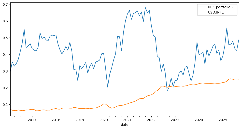
Rolling cumulative return can be helpful in the same situations as rolling CAGR:
[32]:
rf3.get_rolling_cumulative_return(window=12 * 5).plot(); # window size is in months (5 year cumulative return here)
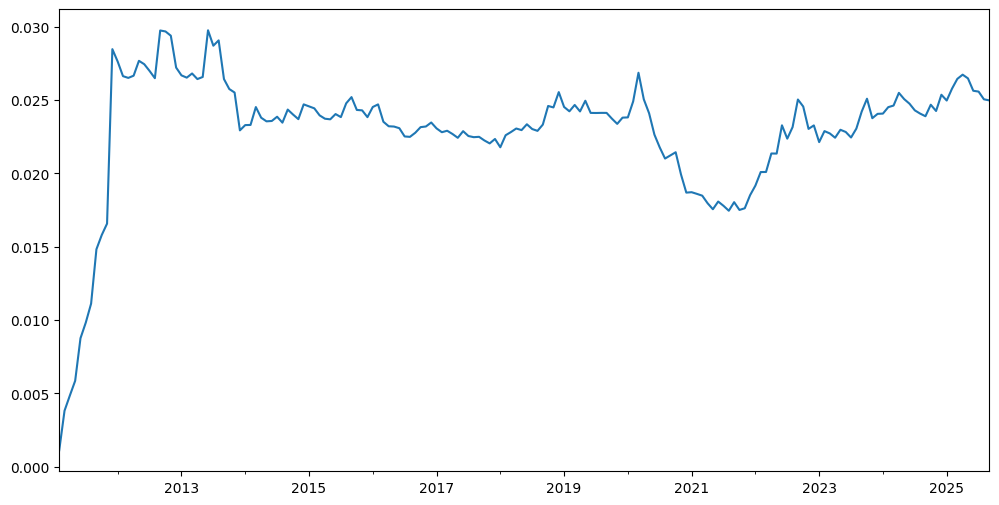
Last-twelve-month (LTM) dividend yield is available through the dividend_yield property.
[33]:
rf3.dividend_yield.plot();
The portfolio also has a monthly dividends time series:
[34]:
rf3.dividends.tail()
[34]:
2025-05     3.416226
2025-06    11.002825
2025-07     3.423926
2025-08     3.529997
2025-09     9.977436
Freq: M, Name: RF3_portfolio.PF, dtype: float64
Calendar-year dividend totals are available for the portfolio:
[35]:
rf3.dividends.resample("Y").sum().plot(kind="bar");
Sharpe Ratio was developed by Nobel laureate William F. Sharpe and is used to understand the return of an investment compared to its risk.
\[S_p = \frac{R_p - R_f}{\sigma_p}\]\(R_p\) - expected return of portfolio
[36]:
rf3.get_sharpe_ratio(rf_return=0.02) # risk-free rate is 2% here
[36]:
np.float64(0.5782476698777302)
Finally, the easiest way to inspect the basic properties of a portfolio is with describe:
[37]:
rf3.describe()
[37]:
| property | period | RF3_portfolio.PF | inflation | |
|---|---|---|---|---|
| 0 | compound return | YTD | 0.134785 | 0.028957 |
| 1 | CAGR | 1 years | 0.117922 | 0.030089 |
| 2 | CAGR | 5 years | 0.082588 | 0.045298 |
| 3 | CAGR | 10 years | 0.083948 | 0.031624 |
| 4 | CAGR | 14 years, 8 months | 0.076007 | 0.026678 |
| 5 | Annualized mean return | 14 years, 8 months | 0.077781 | NaN |
| 6 | Dividend yield | LTM | 0.02497 | NaN |
| 7 | Risk | 14 years, 8 months | 0.099924 | NaN |
| 8 | CVAR (α=1) | 14 years, 8 months | 0.177933 | NaN |
| 9 | Max drawdown | 14 years, 8 months | -0.210563 | NaN |
| 10 | Max drawdown date | 14 years, 8 months | 2022-09 | NaN |
Compare several portfolios
A portfolio is a kind of financial asset and can be included in AssetList to compare it with other portfolios, assets, or benchmarks.
Let’s create Rick Ferri’s four-asset portfolio and compare its behavior with the three-asset portfolio.
[38]:
assets = ["BND.US", "VTI.US", "VXUS.US", "VNQ.US"]  # Vanguard REIT ETF (VNQ) is added.
weights = [0.40, 0.30, 0.24, 0.06]
To compare it properly with RF3, we should choose the same rebalancing period:
[39]:
rf4 = ok.Portfolio(
    assets=assets, weights=weights, rebalancing_strategy=ok.Rebalance(period="year"), symbol="RF4_portfolio.PF"
)  # we also give a custom name to portfolio with 'symbol' propety
rf4
[39]:
symbol                                        RF4_portfolio.PF
assets                       [BND.US, VTI.US, VXUS.US, VNQ.US]
weights                                 [0.4, 0.3, 0.24, 0.06]
rebalancing_period                                        year
rebalancing_abs_deviation                                 None
rebalancing_rel_deviation                                 None
currency                                                   USD
inflation                                             USD.INFL
first_date                                             2011-02
last_date                                              2025-09
period_length                               14 years, 8 months
dtype: object
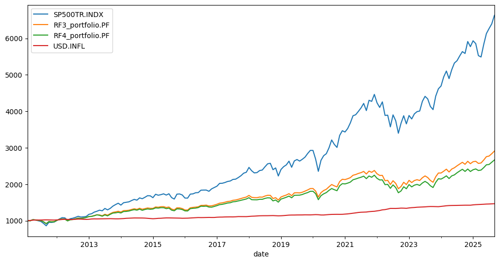
Now we create an AssetList to compare RF3 with RF4 and add a benchmark (the S&P 500 Total Return index).
[40]:
ls = ok.AssetList(["SP500TR.INDX", rf3, rf4])
ls
[40]:
assets           [SP500TR.INDX, RF3_portfolio.PF, RF4_portfolio...
currency                                                       USD
first_date                                                 2011-03
last_date                                                  2025-09
period_length                                   14 years, 7 months
inflation                                                 USD.INFL
dtype: object
Their behavior can be compared with wealth_indexes:
[41]:
ls.wealth_indexes.plot();
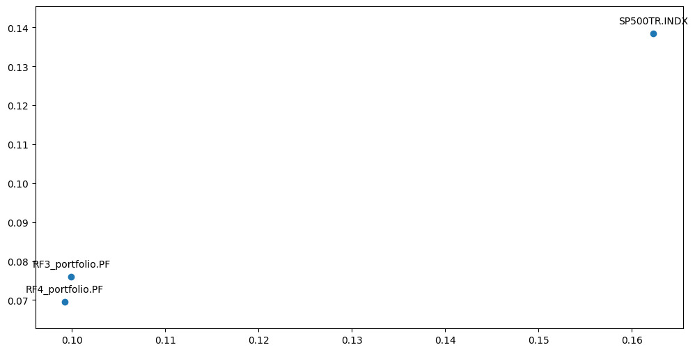
plot_assets. X-axis: Risk (standard deviation)[42]:
ls.plot_assets(kind="cagr"); # set Y-axis to CAGR by kind='cagr'
See06 efficient frontier single period.ipynband07 efficient frontier multi-period.ipynbto plot portfolios together with the Efficient Frontier.
Given a risk-free rate, it is easy to compare the Sharpe ratios of the portfolios with get_sharpe_ratio:
[43]:
ls.get_sharpe_ratio(rf_return=0.02) # Risk-Free rate is 2% here
[43]:
Symbols
SP500TR.INDX        0.742301
RF3_portfolio.PF    0.578248
RF4_portfolio.PF    0.521450
dtype: float64
describe method.YTD (Year to Date) compound return
CAGR for a given list of periods and for the full available history
annualized mean return (arithmetic mean)
LTM dividend yield (last-twelve-month dividend yield)
Risk metrics for the full period:
risk (standard deviation)
CVaR (time frame is 1 year)
maximum drawdowns (and their dates)
[44]:
ls.describe([1, 5, 8]) # portfolio CAGR is shown for YTD, 1, 5, 8 years and for the full histrical period.
[44]:
| property | period | SP500TR.INDX | RF3_portfolio.PF | RF4_portfolio.PF | inflation | |
|---|---|---|---|---|---|---|
| 0 | Compound return | YTD | 0.148334 | 0.134785 | 0.134547 | 0.028957 |
| 1 | CAGR | 1 years | 0.176007 | 0.117922 | 0.105607 | 0.030089 |
| 2 | CAGR | 5 years | 0.164748 | 0.082588 | 0.075639 | 0.045298 |
| 3 | CAGR | 8 years | 0.148874 | 0.078605 | 0.070729 | 0.034951 |
| 4 | CAGR | 14 years, 7 months | 0.138509 | 0.076007 | 0.069573 | 0.026678 |
| 5 | Annualized mean return | 14 years, 7 months | 0.140482 | 0.077781 | 0.071738 | NaN |
| 6 | Dividend yield | LTM | 0.0 | 0.024124 | 0.026396 | NaN |
| 7 | Risk | 14 years, 7 months | 0.162309 | 0.099924 | 0.09922 | NaN |
| 8 | CVAR | 14 years, 7 months | 0.167821 | 0.177933 | 0.181796 | NaN |
| 9 | Max drawdowns | 14 years, 7 months | -0.238631 | -0.210563 | -0.213989 | NaN |
| 10 | Max drawdowns dates | 14 years, 7 months | 2022-09 | 2022-09 | 2022-09 | NaN |
| 11 | Inception date | None | 1988-02 | 2011-02 | 2011-02 | 2011-03 |
| 12 | Last asset date | None | 2025-11 | 2025-09 | 2025-09 | 2025-09 |
| 13 | Common last data date | None | 2025-09 | 2025-09 | 2025-09 | 2025-09 |